Descriptive Analysis of Community Change
For the Descriptive Analysis of Community Change, this part of the project uses:
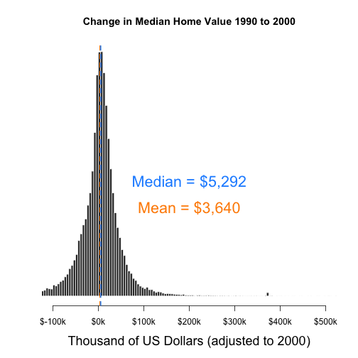
- Census data to calculate change in the MHV (Median Home Values) variable between 1990 and 2000.
- Measure gentrification that occurs between 2000-2010.
- Create a new dorling cartogram to visualize the data for Phoenix Metro Area.
- Prepare descriptive statistics and chloropleth maps describing the MHV change variable, gentrification, and neighborhood health metrics.
Set-Up
Library
# load Library

library(dplyr)  # data wrangling
library(stargazer)  # table formatting
library(scales)  # centers data
library(here)  # creates relative file paths
library(geojsonio)  # read geoJSON map files from GitHub
library(sp)  # spatial data class sp for shapefiles
library(cartogram)  # spatial maps w/ tract size bias reduction
library(tmap)  # thematic maps
library(maptools)  # spatial object manipulation
library(sf)  # 'simple features' flavor of shapefiles

# set stargazer type to text for previewing in RMD docs but convert to type HTML
# when knitting (next code chunk)

s.type <- "html"
Helper Functions
# Load helper functions for graphing purposes

source(here("functions/lab-05_helper_functions_cs.R"))
Data
Load Data sets for 1990 and 2000 and give the number of tracts present.
# load data
d1 <- readRDS(here("data/processed/LTDB-1990.rds"))
d2 <- readRDS(here("data/processed/LTDB-2000.rds"))
md <- readRDS(here("data/processed/LTDB-META-DATA.rds"))


d1 <- select(d1, -year)
d2 <- select(d2, -year)

# merge three tables by tract-id
d <- merge(d1, d2, by = "tractid")
d <- merge(d, md, by = "tractid")

nrow(d)
[1] 72693
Keep only urban data for the analysis
# filter rural districts
table(d$urban.x)
rural urban
12971 59722
d <- filter(d, urban.x == "urban")
Find common variables present in 1990 and 2000 Census Data
# find variables that are in both files
compare_dfs <- function(df1, df2) {
    # use regular expressions to remove numeric suffixes
    var.names.1 <- names(df1)
    var.names.1 <- gsub("[.][xy]$", "", var.names.1)
    var.names.1 <- gsub("[0-9]{2}$", "", var.names.1)

    var.names.2 <- names(df2)
    var.names.2 <- gsub("[.][xy]$", "", var.names.2)
    var.names.2 <- gsub("[0-9]{2}$", "", var.names.2)

    shared <- intersect(var.names.1, var.names.2) %>% sort()
    print("SHARED VARIABLES:")
    print(shared)

    not.shared <- c(setdiff(var.names.1, var.names.2), setdiff(var.names.2, var.names.1)) %>%
        sort()

    print("NOT SHARED:")
    print(not.shared)

    d.vars1 <- data.frame(type = "shared", variables = shared, stringsAsFactors = F)
    d.vars2 <- data.frame(type = "not shared", variables = not.shared, stringsAsFactors = F)
    dd <- rbind(d.vars1, d.vars2)

    return(dd)
}

vars <- compare_dfs(df1 = d1, df2 = d2)
[1] "SHARED VARIABLES:"
 [1] "a15asn" "a15blk" "a15hsp" "a15ntv" "a15wht" "a18und" "a60asn" "a60blk"
 [9] "a60hsp" "a60ntv" "a60up"  "a60wht" "a75up"  "ag15up" "ag25up" "ag5up"
[17] "ageasn" "ageblk" "agehsp" "agentv" "agewht" "asian"  "china"  "clf"
[25] "cni16u" "col"    "cuban"  "dapov"  "dbpov"  "dflabf" "dfmpov" "dhpov"
[33] "dis"    "dmulti" "dnapov" "dpov"   "dwpov"  "empclf" "family" "fb"
[41] "fhh"    "filip"  "flabf"  "geanc"  "gefb"   "h10yrs" "h30old" "haw"
[49] "hh"     "hha"    "hhb"    "hhh"    "hhw"    "hinc"   "hinca"  "hincb"
[57] "hinch"  "hincw"  "hisp"   "hs"     "hu"     "incpc"  "india"  "iranc"
[65] "irfb"   "itanc"  "itfb"   "japan"  "korea"  "lep"    "manuf"  "mar"
[73] "mex"    "mhmval" "mrent"
 [ reached getOption("max.print") -- omitted 32 entries ]
[1] "NOT SHARED:"
[1] "ag16cv"  "ag18cv"  "hu00sp"  "hu90sp"  "ohu00sp" "ohu90sp" "pop90.1"
# list common variable in a table form
head(vars)
    type variables
1 shared    a15asn
2 shared    a15blk
3 shared    a15hsp
4 shared    a15ntv
5 shared    a15wht
6 shared    a18und
d.full <- d # keep a copy so don't have to reload
d <- d.full # store original in case you need to reset anything
Create a subset of data for analysis
# create data set for analysis

d <- select(d, tractid, mhmval90, mhmval90, hinc90, hu90, own90, rent90, empclf90,
    clf90, unemp90, prof90, dpov90, npov90, ag25up90, hs90, col90, pop90.x, nhwht90,
    nhblk90, hisp90, asian90, cbsa.x, cbsaname.x)
d <- d %>% mutate(p.white = 100 * nhwht90/pop90.x, p.black = 100 * nhblk90/pop90.x,
    p.hisp = 100 * hisp90/pop90.x, p.asian = 100 * asian90/pop90.x, p.hs = 100 *
        (hs90 + col90)/ag25up90, p.col = 100 * col90/ag25up90, p.prof = 100 * prof90/empclf90,
    p.unemp = 100 * unemp90/clf90, pov.rate = 100 * npov90/dpov90)
colnames(d)
 [1] "tractid"    "mhmval90"   "hinc90"     "hu90"       "own90"
 [6] "rent90"     "empclf90"   "clf90"      "unemp90"    "prof90"
[11] "dpov90"     "npov90"     "ag25up90"   "hs90"       "col90"
[16] "pop90.x"    "nhwht90"    "nhblk90"    "hisp90"     "asian90"
[21] "cbsa.x"     "cbsaname.x" "p.white"    "p.black"    "p.hisp"
[26] "p.asian"    "p.hs"       "p.col"      "p.prof"     "p.unemp"
[31] "pov.rate"
Regression analysis for variables based on 1990 census data
# regression analysis of the variable

stargazer(d, type = s.type, digits = 0, summary.stat = c("min", "p25", "median",
    "mean", "p75", "max"))
| Statistic | Min | Pctl(25) | Median | Mean | Pctl(75) | Max |
| mhmval90 | 0 | 58,800 | 86,500 | 112,399 | 141,800 | 500,001 |
| hinc90 | 4,999 | 24,355 | 32,033 | 34,160 | 41,520 | 150,001 |
| hu90 | 0 | 916 | 1,337 | 1,382 | 1,804 | 11,003 |
| own90 | 0 | 422 | 744 | 788 | 1,093 | 8,180 |
| rent90 | 0 | 168 | 358 | 476 | 663 | 8,653 |
| empclf90 | 0 | 1,015 | 1,555 | 1,625 | 2,157 | 11,816 |
| clf90 | 0 | 1,101 | 1,664 | 1,732 | 2,291 | 12,497 |
| unemp90 | 0 | 49 | 88 | 107 | 143 | 1,165 |
| prof90 | 0 | 192 | 359 | 451 | 616 | 6,290 |
| dpov90 | 0 | 2,219 | 3,250 | 3,332 | 4,365 | 23,619 |
| npov90 | 0 | 112 | 248 | 406 | 526 | 5,890 |
| ag25up90 | 0 | 1,444 | 2,121 | 2,187 | 2,865 | 18,461 |
| hs90 | 0 | 626 | 1,064 | 1,141 | 1,559 | 12,383 |
| col90 | 0 | 162 | 335 | 483 | 652 | 8,575 |
| pop90.x | 0 | 2,283 | 3,325 | 3,419 | 4,464 | 35,721 |
| nhwht90 | 0 | 1,262 | 2,424 | 2,513 | 3,575 | 21,561 |
| nhblk90 | 0 | 18 | 76 | 426 | 331 | 12,121 |
| hisp90 | 0 | 27 | 75 | 347 | 280 | 13,873 |
| asian90 | 0 | 9 | 31 | 111 | 94 | 7,899 |
| p.white | 0 | 64 | 87 | 74 | 95 | 100 |
| p.black | 0 | 1 | 3 | 12 | 10 | 100 |
| p.hisp | 0 | 1 | 3 | 10 | 9 | 100 |
| p.asian | 0 | 0 | 1 | 3 | 3 | 94 |
| p.hs | 0 | 69 | 74 | 74 | 80 | 100 |
| p.col | 0 | 10 | 18 | 22 | 30 | 100 |
| p.prof | 0 | 17 | 25 | 27 | 34 | 100 |
| p.unemp | 0 | 4 | 5 | 7 | 8 | 64 |
| pov.rate | 0 | 4 | 8 | 12 | 16 | 100 |
Exploration of Median Home value
Intial condition in 1990 after adjusting for inflation.
# intial condition in 1990 adjust 1900 home values for inflation 2.3 % was the
# average inflation rate in 1990, adjusting it to 10 year inflation factor
# (1.023)^10 = 1.255325
d <- d.full
mhv.90 <- d$mhmval90 * 1.255325
mhv.00 <- d$mhmval00

mhv.change <- mhv.00 - mhv.90

df <- data.frame(MedianHomeValue1990 = mhv.90, MedianHomeValue2000 = mhv.00, Change.90.to.00 = mhv.change)

stargazer(df, type = s.type, digits = 0, summary.stat = c("min", "p25", "median",
    "mean", "p75", "max"))
| Statistic | Min | Pctl(25) | Median | Mean | Pctl(75) | Max |
| MedianHomeValue1990 | 0 | 73,813 | 108,586 | 141,098 | 178,005 | 627,664 |
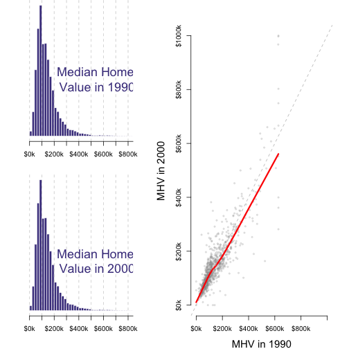
| MedianHomeValue2000 | 0 | 81,600 | 119,900 | 144,738 | 173,894 | 1,000,001 |
| Change.90.to.00 | -627,664 | -15,590 | 5,292 | 3,640 | 24,312 | 1,000,001 |
Histogram representing MHV (absolute value) in 1990
# histogram of MHV

hist(mhv.change/1000, breaks = 500, xlim = c(-100, 500), yaxt = "n", xaxt = "n",
    xlab = "Thousand of US Dollars (adjusted to 2000)", cex.lab = 1.5, ylab = "",
    main = "Change in Median Home Value 1990 to 2000", col = "gray20", border = "white")

axis(side = 1, at = seq(from = -100, to = 500, by = 100), labels = paste0("$", seq(from = -100,
    to = 500, by = 100), "k"))

mean.x <- mean(mhv.change/1000, na.rm = T)
abline(v = mean.x, col = "darkorange", lwd = 2, lty = 2)
text(x = 200, y = 1500, labels = paste0("Mean = ", dollar(round(1000 * mean.x, 0))),
    col = "darkorange", cex = 1.8, pos = 3)

median.x <- median(mhv.change/1000, na.rm = T)
abline(v = median.x, col = "dodgerblue", lwd = 2, lty = 2)
text(x = 200, y = 2000, labels = paste0("Median = ", dollar(round(1000 * median.x,
    0))), col = "dodgerblue", cex = 1.8, pos = 3)
Compare 1990 and 2000 MHV (absolute values)
# compare 1990 and 2000
layout.matrix <- matrix( c( 1,3,
                            2,3 ),
                nrow=2, ncol=2, byrow=T )

layout( mat = layout.matrix,
        heights = c(2,2), # Heights of the two rows
        widths =  c(3,4)) # Widths of the two columns

# layout.show(3)

par( mar=c(4,0,0,2) )

hist( mhv.00/1000, breaks=50,
      xlim=c(-200,800), yaxt="n", xaxt="n",
      xlab="", cex.lab=1,
      ylab="", main="",
      col="darkslateblue", border="white" )

axis( side=1, at=seq( from=0, to=1000, by=100 ),
      labels=paste0( "$", seq( from=0, to=1000, by=100 ), "k" ) )

abline( v=seq(0,1000,100), lty=2, col="gray80" )

text( 550, 4000, labels="Median Home \nValue in 1990",
      col="darkslateblue", cex=1.8 )


hist( mhv.00/1000, breaks=50,
      xlim=c(-200,800), yaxt="n", xaxt="n",
      xlab="", cex.lab=1,
      ylab="", main="",
      col="darkslateblue", border="white" )

abline( v=seq(0,1000, 100 ), lty=2, col="gray80" )

text( 550, 3500, labels="Median Home \nValue in 2000",
      col="darkslateblue", cex=1.8 )

axis( side=1, at=seq( from=0, to=1000, by=100 ),
      labels=paste0( "$", seq( from=0, to=1000, by=100 ), "k" ) )


# data reduction - filter 1,000 observations

df <- data.frame( v90=mhv.90/1000, v00=mhv.00/1000 )
df <- sample_n( df, 1000 )

par( mar=c(4,5,3,2) )

jplot( df$v90, df$v00,
       lab1="MHV in 1990", lab2="MHV in 2000",
       xlim=c(0,1000), ylim=c(0,1000),
       axes=F )

abline( a=0, b=1, lty=2, col="gray" )
axis( side=1, at=seq( from=0, to=1000, by=200 ),
      labels=paste0( "$", seq( from=0, to=1000, by=200 ), "k" ) )
axis( side=2, at=seq( from=0, to=1000, by=200 ),
      labels=paste0( "$", seq( from=0, to=1000, by=200 ), "k" ) )
Calculate summary table for percentage change in MHV 1990 and 2000
# % change in MHV 1990 and 2000
mhv.90[mhv.90 < 1000] <- NA
pct.change <- mhv.change/mhv.90
summary(pct.change)
     Min.   1st Qu.    Median      Mean   3rd Qu.      Max.      NA's
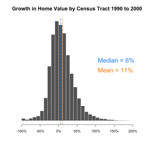
 -1.00000  -0.11611   0.05614   0.10823   0.26418 214.79478       141
Number of tracts to experience more than 500% change in MHV
# how many cases had increases above 500%
sum(pct.change > 5, na.rm = T)
[1] 30
Showing 6 of 30 tracts to experience more than 500% change in MHV
# preview tracts with large increases in home values to see if increases make
# sense

d %>% filter(pct.change > 5) %>% head()
     tractid pop90.x nhwht90 nhblk90 ntv90 asian90 hisp90 haw90 india90 china90
     filip90 japan90 korea90 viet90 mex90 pr90 cuban90 hu90 vac90 ohu90
     a18und90 a60up90 a75up90 agewht90 a15wht90 a60wht90 ageblk90 a15blk90
     a60blk90 agehsp90 a15hsp90 a60hsp90 agentv90 a15ntv90 a60ntv90 ageasn90
     a15asn90 a60asn90 ag15up90 mar90 wds90 mhmval90 mrent90 own90 rent90
     family90 fhh90 pop90.y pop90.1 ruanc90 itanc90 geanc90 iranc90 scanc90
     rufb90 itfb90 gefb90 irfb90 scfb90 fb90 nat90 n10imm90 ag5up90 olang90
     lep90 ag25up90 hs90 col90 clf90 unemp90 dflabf90 flabf90 empclf90 prof90
     manuf90 semp90 ag16cv90 vet90 cni16u90 dis90 dpov90 npov90 n65pov90
     dfmpov90 nfmpov90 dwpov90 nwpov90 dbpov90 nbpov90 dnapov90 nnapov90
     dhpov90 nhpov90 dapov90 napov90 incpc90 hu90sp h30old90 ohu90sp h10yrs90
     dmulti90 multi90 hinc90 hincw90 hincb90 hinch90 hinca90 hh90 hhw90 hhb90
     hhh90 hha90 pop00.x nhwht00 nhblk00 ntv00 asian00 hisp00 haw00 india00
     china00 filip00 japan00 korea00 viet00 mex00 pr00 cuban00 hu00 vac00 ohu00
     a18und00 a60up00 a75up00 agewht00 a15wht00 a60wht00 ageblk00 a15blk00
     a60blk00 agehsp00 a15hsp00 a60hsp00 agentv00 a15ntv00 a60ntv00 ageasn00
     a15asn00 a60asn00 family00 fhh00 own00 rent00 pop00.y ruanc00 itanc00
     geanc00 iranc00 scanc00 rufb00 itfb00 gefb00 irfb00 scfb00 fb00 nat00
     n10imm00 ag5up00 olang00 lep00 ag25up00 hs00 col00 ag15up00 mar00 wds00
     clf00 unemp00 dflabf00 flabf00 empclf00 prof00 manuf00 semp00 ag18cv00
     vet00 cni16u00 dis00 dpov00 npov00 n65pov00 dfmpov00 nfmpov00 dwpov00
     nwpov00 dbpov00 nbpov00 dnapov00 nnapov00 dhpov00 nhpov00 dapov00 napov00
     incpc00 hu00sp h30old00 ohu00sp h10yrs00 dmulti00 multi00 hinc00 hincw00
     hincb00 hinch00 hinca00 mhmval00 mrent00 hh00 hhw00 hhb00 hhh00 hha00
     fipscounty state county tract placefp10 cbsa10 metdiv10 ccflag10 globd00
     globg00 globd90 globg90 globd80 globg80 msa.x msaname.x cbsa.x cbsaname.x
     urban.x msa.y msaname.y cbsa.y cbsaname.y urban.y
 [ reached 'max' / getOption("max.print") -- omitted 6 rows ]
Plot to show percentage change in MHV between 1990-2000
# Plot the percent change variable:
hg <- hist(pct.change, breaks = 2000, xlim = c(-1, 2), yaxt = "n", xaxt = "n", xlab = "",
    cex.main = 1.5, ylab = "", main = "Growth in Home Value by Census Tract 1990 to 2000",
    col = "gray40", border = "white")

axis(side = 1, at = seq(from = -1, to = 2, by = 0.5), labels = paste0(seq(from = -100,
    to = 200, by = 50), "%"))

ymax <- max(hg$count)

mean.x <- mean(pct.change, na.rm = T)
abline(v = mean.x, col = "darkorange", lwd = 2, lty = 2)
text(x = 1, y = (0.5 * ymax), labels = paste0("Mean = ", round(100 * mean.x, 0),
    "%"), col = "darkorange", cex = 1.8, pos = 4)

median.x <- median(pct.change, na.rm = T)
abline(v = median.x, col = "dodgerblue", lwd = 2, lty = 2)
text(x = 1, y = (0.6 * ymax), labels = paste0("Median = ", round(100 * median.x,
    0), "%"), col = "dodgerblue", cex = 1.8, pos = 4)
Group Growth Rate by Metro-area for the time period 1990-2000 (showing highest 25)
# Group Growth Rates By Metro Area
d$mhv.change <- mhv.change
d$pct.change <- pct.change
d$mhv.00 <- mhv.00
d$mhv.90 <- mhv.90

d %>% group_by(cbsaname.x) %>% summarize(ave.change = median(mhv.change, na.rm = T),
    ave.change.d = dollar(round(ave.change, 0)), growth = 100 * median(pct.change,
        na.rm = T)) %>% ungroup() %>% arrange(-growth) %>% select(-ave.change) %>%
    head(25)
# A tibble: 25 x 3
   cbsaname.x                          ave.change.d growth
   <chr>                               <chr>         <dbl>
 1 Corvallis, OR                       $78,276        84.5
 2 Portland-Vancouver-Beaverton, OR-WA $72,661        80.6
 3 Salt Lake City, UT                  $65,864        77.7
 4 Boulder, CO                         $101,351       77.2
 5 Provo-Orem, UT                      $64,922        76.5
 6 Salem, OR                           $52,248        69.6
 7 Eugene-Springfield, OR              $55,029        69.4
 8 Fort Collins-Loveland, CO           $61,268        64.4
 9 Longview, WA                        $44,733        63.0
10 Missoula, MT                        $49,358        62.3
# … with 15 more rows
Analysis
How do changes in home value differ between the 1990-2000 period and 2000-2010?
The changes in home value between 1990-2000 and 2000-2010 are very different. 2000-2010 has witnessed some of the major historic economic events. The tech-bubble and housing-bubble in early and mid part of this decade has shaped the changes in housing market as well. 2005 witnesses United States Housig market correction, even after the correction the changes in home value between 2000-2010 was significantly higher than 1990-2000.
The changes in MHV in absolute terms 1990-2000 was $3,640 in terms of mean value and $5,292 in terms of median value. The same values for 2000-2010 were $60,047 and $36,268. The mean is greater than the median which shows that the data is skewed toward the right.
The percentage change in MHV which offers more meaningful picture of the change shows that between 1990-2000 the mean change in percent of MHV was 10.82% while between 2000-2010 it was 33.80%. The percentage in the median price was 5.61% and 25.40% respectively.
The difference in the nature of changes in home value is further observed while comparing the number of tracts to witness changes greater than 500%. Between 1990-2000 there were only 30 such tracts whereas between 2000-2010 there were 115.
What do the authors suggest would predict fall in central city home values between 1990 and 2000?
According to Baum-Snow & Hartley, "Accounting for central neighborhood change, 1980-2010", 2016 the census variable which can predict the fall in central city home values between 1990-2000 are:
- Percent of population with High school diploma or less
- Percent of umemployed population
- Percent of white population.
A decline in residents without college degree because of the decline in job opportunities for lesser skilled workers in urban areas caused such population to move out. According to the article lesser skilled white population moved out so a decrease in white population during the period is measured in population loss. Less population translates into less demand for housing which in turn means fall in housing value. So analysing these variables would predict the fall in home values between 1990 and 2000 in urban areas.
Change in Neighborhood Vitality
Data
Load data sets for 2000 and 2010 and give the number of tracts present
# load data

d3 <- readRDS(here("data/processed/LTDB-2000.rds"))
d4 <- readRDS(here("data/processed/LTDB-2010.rds"))
md <- readRDS(here("data/processed/LTDB-META-DATA.rds"))


d3 <- select(d3, -year)
d4 <- select(d4, -year)

# merge three tables by tract-id
d5 <- merge(d3, d4, by = "tractid")
d5 <- merge(d5, md, by = "tractid")

nrow(d4)
[1] 74022
Keep only urban data
# filter rural districts
table(d$urban.x)
urban
59722
d5 <- filter(d5, urban.x == "urban")
d.full1 <- d5 # keep a copy so don't have to reload
d5 <- d.full1 # story original in case you need to reset anything
Create a subset of data for analysis and select variable needed to observe neighborhood vitality
# create data set for analysis

d5 <- select(d5, tractid, mhmval00, mhmval12, prof00, prof12, hinc00, hinc12, col00,
    col12, incpc00, incpc12, hs00, hs12, unemp00, unemp12, wds00, wds12, clf00, cbsa.x,
    cbsaname.x, ag25up00, empclf00, empclf12, ag25up12, clf12, ag15up12, ag15up00) %>%
    filter(incpc00 != 0, ag25up00 != 0, ag25up12 != 0, empclf00 != 0, empclf12 !=
        0, clf00 != 0, clf12 != 0, ag15up00 != 0, ag15up12 != 0, prof00 != 0, prof12 !=
        0, col00 != 0, col12 != 0, hs00 != 0, hs12 != 0, unemp00 != 0, unemp12 !=
        0, wds00 != 0, wds12 != 0)
d5 <- d5 %>% mutate(p.hs.00 = 100 * (hs00 + col00)/ag25up00, p.hs.10 = 100 * (hs12 +
    col12)/ag25up12, p.col.00 = 100 * col00/ag25up00, p.col.10 = 100 * col12/ag25up12,
    p.prof.00 = 100 * prof00/empclf00, p.prof.10 = 100 * prof12/empclf12, p.unemp.00 = 100 *
        unemp00/clf00, p.unemp.10 = 100 * unemp12/clf12, p.wds.00 = 100 * wds00/ag15up00,
    p.wds.10 = 100 * wds12/ag15up12) %>%
mutate_if(is.numeric, list(~na_if(., Inf))) %>% mutate_if(is.numeric, list(~na_if(.,
    -Inf))) %>%
na.omit()
Regression analysis of the variables in 2000 and 2010
reg.data.00 <- d5 %>% select(mhmval00, mhmval12, hinc00, hinc12, incpc00, incpc12,
    p.hs.00, p.hs.10, p.col.00, p.col.10, p.prof.00, p.prof.10, p.unemp.00, p.unemp.10,
    p.wds.00, p.wds.10)
stargazer(reg.data.00, type = s.type, digits = 0, summary.stat = c("min", "p25",
    "median", "mean", "p75"))
| Statistic | Min | Pctl(25) | Median | Mean | Pctl(75) |
| mhmval00 | 0 | 81,700 | 119,800 | 144,714 | 174,000 |
| mhmval12 | 9,999 | 122,500 | 191,000 | 246,312 | 313,325 |
| hinc00 | 2,797 | 33,000 | 43,761 | 47,665 | 58,069 |
| hinc12 | 2,499 | 39,124 | 53,918 | 59,549 | 73,792 |
| incpc00 | 1,866 | 15,788 | 20,522 | 22,668 | 26,604 |
| incpc12 | 1,269 | 19,301 | 26,102 | 29,122 | 35,005.2 |
| p.hs.00 | 26 | 67 | 72 | 72 | 77 |
| p.hs.10 | 25 | 66 | 71 | 71 | 77 |
| p.col.00 | 0 | 12 | 21 | 26 | 36 |
| p.col.10 | 0 | 15 | 25 | 30 | 41 |
| p.prof.00 | 1 | 23 | 31 | 34 | 43 |
| p.prof.10 | 0 | 24 | 34 | 35 | 46 |
| p.unemp.00 | 0 | 3 | 5 | 6 | 8 |
| p.unemp.10 | 0 | 6 | 9 | 10 | 13 |
| p.wds.00 | 0 | 14 | 18 | 19 | 22 |
| p.wds.10 | 0 | 15 | 19 | 19 | 23 |
Initial regression in 2000
# median home value in 2000, 2010, change and percentage change 2000 values
# adjusted for inflation
mhmval.00 <- d5$mhmval00 * 1.28855
mhmval.10 <- d5$mhmval12
mhmval.change <- mhmval.10 - mhmval.00
pct.mhmval <- mhmval.change/mhmval.00

# Percapita income in 2000, 2010, change and percentage chnage 2000 values
# adjusted for inflation
incp.00 <- d5$incpc00 * 1.28855
incpc.10 <- d5$incpc12
incpc.change <- incpc.10 - incp.00
pct.incpc.change <- incpc.change/incp.00

# Median House Hold income income in 2000, 2010, change and percentage chnage
# 2000 values adjusted for inflation
hinc.00 <- d5$hinc00 * 1.28855
hinc.10 <- d5$hinc12
hinc.change <- hinc.10 - hinc.00
pct.hinc.change <- hinc.change/hinc.00

# % of professional employees in 2000, 2010, change and percentage chnage
pprof.00 <- d5$p.prof.00
pprof.10 <- d5$p.prof.10
pprof.change <- pprof.10 - pprof.00
pct.pprof.change <- pprof.change/pprof.00

# % of popualtion with High school degree or less in 2000, 2010, change and
# percentage chnage
phs.00 <- d5$p.hs.00
phs.10 <- d5$p.hs.10
phs.change <- phs.10 - phs.00
pct.phs.change <- phs.change/phs.00
# % of population with four years of college or more in 2000, 2010, change and
# percentage chnage
pcol.00 <- d5$p.col.00
pcol.10 <- d5$p.col.10
pcol.change <- pcol.10 - pcol.00
pct.pcol.change <- pcol.change/pcol.00

# % of unemployed population in 2000, 2010, change and percentage chnage
punemp.00 <- d5$p.unemp.00
punemp.10 <- d5$p.unemp.10
punemp.change <- punemp.10 - punemp.00
pct.punemp.change <- punemp.change/punemp.00

# % of widowed, divorced and single population in 2000, 2010, change and
# percentage chnage
pwds.00 <- d5$p.wds.00
pwds.10 <- d5$p.wds.10
pwds.change <- pwds.10 - pwds.00
pct.pwds.change <- pwds.change/pwds.00

df1 <- data.frame(MedianHomeValue2000 = mhmval.00, MedianHomeValue2010 = mhmval.10,
    PercentGrowthMedianHomeValue.00.to.10 = pct.mhmval, HouseHoldIncome2000 = hinc.00,
    HouseHoldIncome2010 = hinc.10, HouseHoldIncomeChange.00.to.10 = hinc.change,
    PerCapitaIncome2000 = incp.00, PerCapitaIncome2010 = incpc.10, PerCaptiaIncomeChange.00.to.10 = incpc.change,
    PercentOfProfessionalEmployyes2000 = pprof.00, PercentOfProfessionalEmployyes2010 = pprof.10,
    ProfessionalChange.00.to.10 = pct.pprof.change, PercentWithHighSchoolDegreeOrLess2000 = phs.00,
    PercentWithHighSchoolDegreeOrLess2010 = phs.00, PercentWithHighSchoolDegreeOrLessChange.00.to.10 = pct.phs.change,
    PercentWithFourYearCollegeDegreeOrMore2000 = pcol.00, PercentWithFourYearCollegeDegreeOrMore2010 = pcol.10,
    PercentWithFourYearCollegeDegreeOrMoreChange00.to.10 = pct.pcol.change, Percentunemployed2000 = punemp.00,
    Percentunemployed2010 = punemp.10, PercentunemployedChange.00to.10 = pct.punemp.change,
    PercentWidowedDivorced2000 = pwds.00, PercentWidowedDivorced2010 = pwds.10, PercentWidowedDivorcedChange.00.to.1o = pct.pwds.change) %>%

mutate_if(is.numeric, list(~na_if(., Inf))) %>% mutate_if(is.numeric, list(~na_if(.,
    -Inf))) %>% na.omit()


df.initial <- data.frame(MedianHomevalue2000 = mhmval.00, HouseHoldIncome2000 = hinc.00,
    PerCapitaIncome2000 = incp.00, PercentOfProfessionalEmployyes2000 = pprof.00,
    PercentWithHighSchoolDegreeOrLess2000 = phs.00, PercentWithFourYearCollegeDegreeOrMore2000 = pcol.00,
    Percentunemployed2000 = punemp.00, PercentWidowedDivorced2000 = pwds.00) %>%
    mutate_if(is.numeric, list(~na_if(., Inf))) %>% mutate_if(is.numeric, list(~na_if(.,
    -Inf))) %>% na.omit()

stargazer(df.initial, type = s.type, digits = 0, summary.stat = c("min", "p25", "median",
    "mean", "p75", "max"))
| Statistic | Min | Pctl(25) | Median | Mean | Pctl(75) | Max |
| MedianHomevalue2000 | 0 | 105,275 | 154,368 | 186,471 | 224,208 | 1,288,551 |
| HouseHoldIncome2000 | 3,604 | 42,522 | 56,389 | 61,418 | 74,824 | 257,711 |
| PerCapitaIncome2000 | 2,404 | 20,344 | 26,443 | 29,209 | 34,281 | 214,960 |
| PercentOfProfessionalEmployyes2000 | 1 | 23 | 31 | 34 | 43 | 98 |
| PercentWithHighSchoolDegreeOrLess2000 | 26 | 67 | 72 | 72 | 77 | 100 |
| PercentWithFourYearCollegeDegreeOrMore2000 | 0 | 12 | 21 | 26 | 36 | 95 |
| Percentunemployed2000 | 0 | 3 | 5 | 6 | 8 | 97 |
| PercentWidowedDivorced2000 | 0 | 14 | 18 | 19 | 22 | 70 |
Visualizations of changes from 2000 - 2010
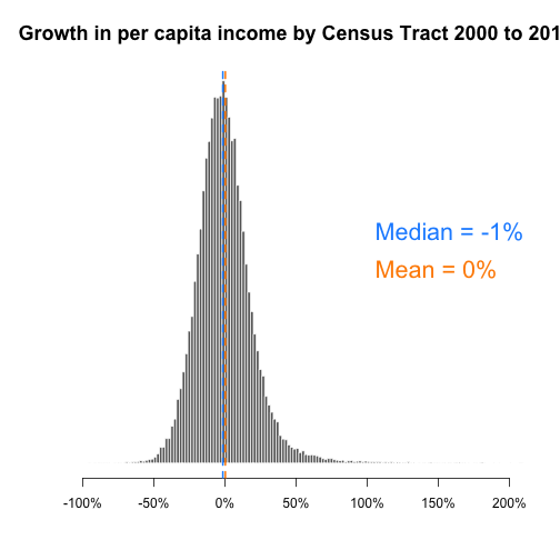
Histogram showing percentage growth in per capita income from 2000-2010
hg2 <- hist(pct.incpc.change, breaks = 2000, xlim = c(-1, 2), yaxt = "n", xaxt = "n",
    xlab = "", cex.main = 1.5, ylab = "", main = "Growth in per capita income by Census Tract 2000 to 2010",
    col = "gray40", border = "white")

axis(side = 1, at = seq(from = -1, to = 2, by = 0.5), labels = paste0(seq(from = -100,
    to = 200, by = 50), "%"))

ymax <- max(hg2$count)

mean.x <- mean(pct.incpc.change, na.rm = T)
abline(v = mean.x, col = "darkorange", lwd = 2, lty = 2)
text(x = 1, y = (0.5 * ymax), labels = paste0("Mean = ", round(100 * mean.x, 0),
    "%"), col = "darkorange", cex = 1.8, pos = 4)

median.x <- median(pct.incpc.change, na.rm = T)
abline(v = median.x, col = "dodgerblue", lwd = 2, lty = 2)
text(x = 1, y = (0.6 * ymax), labels = paste0("Median = ", round(100 * median.x,
    0), "%"), col = "dodgerblue", cex = 1.8, pos = 4)
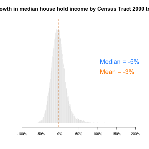
Histogram showing percentage growth in Median Household Income 2000-2010
hg3 <- hist(pct.hinc.change, breaks = 2000, xlim = c(-1, 2), yaxt = "n", xaxt = "n",
    xlab = "", cex.main = 1.5, ylab = "", main = "Growth in median house hold income by Census Tract 2000 to 2010",
    col = "gray40", border = "white")

axis(side = 1, at = seq(from = -1, to = 2, by = 0.5), labels = paste0(seq(from = -100,
    to = 200, by = 50), "%"))

ymax <- max(hg3$count)

mean.x <- mean(pct.hinc.change, na.rm = T)
abline(v = mean.x, col = "darkorange", lwd = 2, lty = 2)
text(x = 1, y = (0.5 * ymax), labels = paste0("Mean = ", round(100 * mean.x, 0),
    "%"), col = "darkorange", cex = 1.8, pos = 4)

median.x <- median(pct.hinc.change, na.rm = T)
abline(v = median.x, col = "dodgerblue", lwd = 2, lty = 2)
text(x = 1, y = (0.6 * ymax), labels = paste0("Median = ", round(100 * median.x,
    0), "%"), col = "dodgerblue", cex = 1.8, pos = 4)
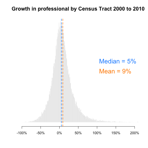
Histogram showing percentage growth in Professionals from 2000-2010
hg4 <- hist(pct.pprof.change, breaks = 20000, xlim = c(-1, 2), yaxt = "n", xaxt = "n",
    xlab = "", cex.main = 1.5, ylab = "", main = "Growth in professional by Census Tract 2000 to 2010",
    col = "gray40", border = "white")

axis(side = 1, at = seq(from = -1, to = 2, by = 0.5), labels = paste0(seq(from = -100,
    to = 200, by = 50), "%"))

ymax <- max(hg4$count)

mean.x <- mean(pct.pprof.change, na.rm = T)
abline(v = mean.x, col = "darkorange", lwd = 2, lty = 2)
text(x = 1, y = (0.5 * ymax), labels = paste0("Mean = ", round(100 * mean.x, 0),
    "%"), col = "darkorange", cex = 1.8, pos = 4)

median.x <- median(pct.pprof.change, na.rm = T)
abline(v = median.x, col = "dodgerblue", lwd = 2, lty = 2)
text(x = 1, y = (0.6 * ymax), labels = paste0("Median = ", round(100 * median.x,
    0), "%"), col = "dodgerblue", cex = 1.8, pos = 4)
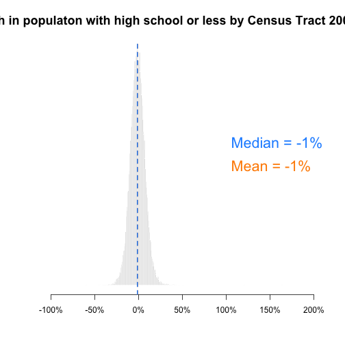
Histogram showing percentage growth in populaton with high school or less by Census Tract 2000 to 2010
hg5 <- hist(pct.phs.change, breaks = 500, xlim = c(-1, 2), yaxt = "n", xaxt = "n",
    xlab = "", cex.main = 1.5, ylab = "", main = "Growth in populaton with high school or less by Census Tract 2000 to 2010",
    col = "gray40", border = "white")

axis(side = 1, at = seq(from = -1, to = 2, by = 0.5), labels = paste0(seq(from = -100,
    to = 200, by = 50), "%"))

ymax <- max(hg5$count)

mean.x <- mean(pct.phs.change, na.rm = T)
abline(v = mean.x, col = "darkorange", lwd = 2, lty = 2)
text(x = 1, y = (0.5 * ymax), labels = paste0("Mean = ", round(100 * mean.x, 0),
    "%"), col = "darkorange", cex = 1.8, pos = 4)

median.x <- median(pct.phs.change, na.rm = T)
abline(v = median.x, col = "dodgerblue", lwd = 2, lty = 2)
text(x = 1, y = (0.6 * ymax), labels = paste0("Median = ", round(100 * median.x,
    0), "%"), col = "dodgerblue", cex = 1.8, pos = 4)
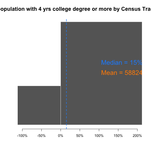
Histogram showing growth in population with 4 yr college degree or more by census tract 2000 to 2010
hg6 <- hist(pct.pcol.change, breaks = 500, xlim = c(-1, 2), yaxt = "n", xaxt = "n",
    xlab = "", cex.main = 1.5, ylab = "", main = "Growth in population with 4 yrs college degree or more by Census Tract 2000 to 2010",
    col = "gray40", border = "white")

axis(side = 1, at = seq(from = -1, to = 2, by = 0.5), labels = paste0(seq(from = -100,
    to = 200, by = 50), "%"))

ymax <- max(hg6$count)

mean.x <- mean(pct.pcol.change, na.rm = T)
abline(v = mean.x, col = "darkorange", lwd = 2, lty = 2)
text(x = 1, y = (0.5 * ymax), labels = paste0("Mean = ", round(100 * mean.x, 0),
    "%"), col = "darkorange", cex = 1.8, pos = 4)

median.x <- median(pct.pcol.change, na.rm = T)
abline(v = median.x, col = "dodgerblue", lwd = 2, lty = 2)
text(x = 1, y = (0.6 * ymax), labels = paste0("Median = ", round(100 * median.x,
    0), "%"), col = "dodgerblue", cex = 1.8, pos = 4)
Histogram showing growth in unemployed population by census tract 2000 to 2010
hg7 <- hist(pct.punemp.change, breaks = 2000, xlim = c(-1, 2), yaxt = "n", xaxt = "n",
    xlab = "", cex.main = 1.5, ylab = "", main = "Growth in unemployed  population by Census Tract 2000 to 2010",
    col = "gray40", border = "white")

axis(side = 1, at = seq(from = -1, to = 2, by = 0.5), labels = paste0(seq(from = -100,
    to = 200, by = 50), "%"))

ymax <- max(hg7$count)

mean.x <- mean(pct.punemp.change, na.rm = T)
abline(v = mean.x, col = "darkorange", lwd = 2, lty = 2)
text(x = 1, y = (0.5 * ymax), labels = paste0("Mean = ", round(100 * mean.x, 0),
    "%"), col = "darkorange", cex = 1.8, pos = 4)

median.x <- median(pct.punemp.change, na.rm = T)
abline(v = median.x, col = "dodgerblue", lwd = 2, lty = 2)
text(x = 1, y = (0.6 * ymax), labels = paste0("Median = ", round(100 * median.x,
    0), "%"), col = "dodgerblue", cex = 1.8, pos = 4)
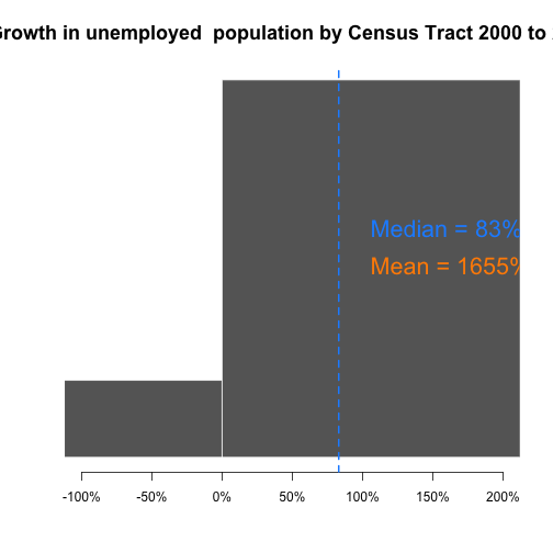
Histogram showing growth in widowed, divorced and single population by Census Tract 2000 to 2010
hg8 <- hist(pct.pwds.change, breaks = 2000, xlim = c(-1, 2), yaxt = "n", xaxt = "n",
    xlab = "", cex.main = 1.5, ylab = "", main = "Growth in widowed, divorced and single population by Census Tract 2000 to 2010",
    col = "gray40", border = "white")

axis(side = 1, at = seq(from = -1, to = 2, by = 0.5), labels = paste0(seq(from = -100,
    to = 200, by = 50), "%"))

ymax <- max(hg8$count)

mean.x <- mean(pct.pwds.change, na.rm = T)
abline(v = mean.x, col = "darkorange", lwd = 2, lty = 2)
text(x = 1, y = (0.5 * ymax), labels = paste0("Mean = ", round(100 * mean.x, 0),
    "%"), col = "darkorange", cex = 1.8, pos = 4)

median.x <- median(pct.pwds.change, na.rm = T)
abline(v = median.x, col = "dodgerblue", lwd = 2, lty = 2)
text(x = 1, y = (0.6 * ymax), labels = paste0("Median = ", round(100 * median.x,
    0), "%"), col = "dodgerblue", cex = 1.8, pos = 4)
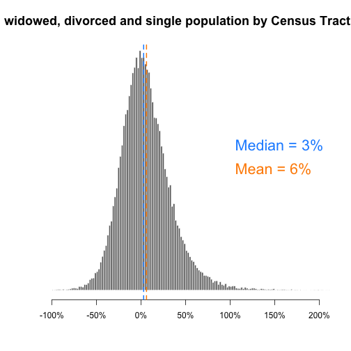
Statistical summary of neighborhood vitality variable from 2000 -2010
summary.df <- data.frame(mhmval.change, pct.hinc.change, pct.incpc.change, pct.pcol.change,
    pct.pprof.change, pct.phs.change, pct.punemp.change, pct.pwds.change)
summary(summary.df)
 mhmval.change      pct.hinc.change    pct.incpc.change   pct.pcol.change
 Min.   :-1063342   Min.   :-0.96352   Min.   :-0.95520   Min.   :      -1
 1st Qu.:    7102   1st Qu.:-0.15841   1st Qu.:-0.12464   1st Qu.:       0
 Median :   35732   Median :-0.04704   Median :-0.01434   Median :       0
 Mean   :   59841   Mean   :-0.02816   Mean   : 0.00337   Mean   :     588
 3rd Qu.:   94150   3rd Qu.: 0.07274   3rd Qu.: 0.10249   3rd Qu.:       0
 Max.   : 1000001   Max.   : 7.55611   Max.   :33.72376   Max.   :33808892
 pct.pprof.change   pct.phs.change     pct.punemp.change  pct.pwds.change
 Min.   :-0.98530   Min.   :-0.59664   Min.   :    -1.0   Min.   :-0.99579
 1st Qu.:-0.08802   1st Qu.:-0.06611   1st Qu.:     0.2   1st Qu.:-0.12861
 Median : 0.05213   Median :-0.01275   Median :     0.8   Median : 0.03012
 Mean   : 0.08979   Mean   :-0.01166   Mean   :    16.6   Mean   : 0.06221
 3rd Qu.: 0.20923   3rd Qu.: 0.04116   3rd Qu.:     1.7   3rd Qu.: 0.21232
 Max.   :90.40845   Max.   : 1.74184   Max.   :490464.0   Max.   :36.61784
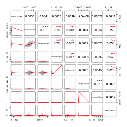
Correlation between changes in neighborhood health metrics and change in home value
Bivariate correlation table of variables
correlation.df <- dplyr::select(df1, "PercentGrowthMedianHomeValue.00.to.10", "HouseHoldIncomeChange.00.to.10",
    "PerCaptiaIncomeChange.00.to.10", "ProfessionalChange.00.to.10", "PercentWithHighSchoolDegreeOrLessChange.00.to.10",
    "PercentWithFourYearCollegeDegreeOrMoreChange00.to.10", "PercentunemployedChange.00to.10",
    "PercentWidowedDivorcedChange.00.to.1o")

pairs(correlation.df, lower.panel = panel.smooth, upper.panel = panel.cor)
Analysis
Do patterns of neighborhood vitality follow the same patterns as home values? Do we see consistent increases over time? What percentage of tracts improved, according to your measures, and what percentage got worse?
The patterns of neighborhood vitality follow the same patterns as home values, most of the variable with exceptions to household income and less educated population see an increase over the period of time.
What is the correlation between change in neighborhood health metrics and change in home value? Consider using the pairs() function from the previous lab to describe these relationships.
The correlation between changes in neighborhood health metrics and changes in home value is shown above in a correlation table.
Measuring Gentrification
Load data
d2 <- d.full
# adjust 1990 home values for inflation average inflation for 1990 is set to
# 2.30% adjusting that for 10 year (1.023)^10 = 1.255325
mhv.90 <- d2$mhmval90 * 1.255325
mhv.00 <- d2$mhmval00

mhv.change <- mhv.00 - mhv.90

# small initial values are skewing percentages an average home value below $10k
# is really low - these must be mostly vacant lots?

mhv.90[mhv.90 < 1000] <- NA
pct.change <- 100 * (mhv.change/mhv.90)
summary(pct.change)
     Min.   1st Qu.    Median      Mean   3rd Qu.      Max.      NA's
 -100.000   -11.611     5.614    10.823    26.418 21479.478       141
d2$mhv.90 <- mhv.90
d2$mhv.00 <- mhv.00
d2$mhv.change <- mhv.change
d2$pct.change <- pct.change
Select variables for operationalizing a definition of gentrification
d2 <- select( d2,

             tractid, cbsa.x, cbsaname.x,            # ids / units of analysis

             mhv.90, mhv.00, mhv.change, pct.change,    # home value

             hinc90, hu90, own90, rent90,        # ses
             hinc00, hu00, own00, rent00,

             empclf90, clf90, unemp90, prof90,   # employment
             empclf00, clf00, unemp00, prof00,

             dpov90, npov90,                     # poverty
             dpov00, npov00,

             ag25up90, hs90, col90,              # education
             ag25up00, hs00, col00,

             pop90.x, nhwht90, nhblk90, hisp90, asian90,   # race
             pop00.y, nhwht00, nhblk00, hisp00, asian00

          ) # end select


d2 <-
  d2 %>%
  mutate(
          # 1990 variables
          p.white.90 = 100 * nhwht90 / pop90.x,
          p.black.90 = 100 * nhblk90 / pop90.x,
          p.hisp.90 = 100 * hisp90 / pop90.x,
          p.asian.90 = 100 * asian90 / pop90.x,
          p.hs.edu.90 = 100 * (hs90+col90) / ag25up90,
          p.col.edu.90 = 100 * col90 / ag25up90,
          p.prof.90 = 100 * prof90 / empclf90,
          p.unemp.90 = 100 * unemp90 / clf90,
          pov.rate.90 = 100 * npov90 / dpov90,

          # 2000 variables
          p.white.00 = 100 * nhwht00 / pop00.y,
          p.black.00 = 100 * nhblk00 / pop00.y,
          p.hisp.00 = 100 * hisp00 / pop00.y,
          p.asian.00 = 100 * asian00 / pop00.y,
          p.hs.edu.00 = 100 * (hs00+col00) / ag25up00,
          p.col.edu.00 = 100 * col00 / ag25up00,
          p.prof.00 = 100 * prof00 / empclf00,
          p.unemp.00 = 100 * unemp00 / clf00,
          pov.rate.00 = 100 * npov00 / dpov00 )
d2 <- d2 %>% group_by(cbsaname.x) %>% mutate(metro.mhv.pct.90 = ntile(mhv.90, 100),
    metro.mhv.pct.00 = ntile(mhv.00, 100), metro.median.pay.90 = median(hinc90, na.rm = T),
    metro.median.pay.00 = median(hinc00, na.rm = T), metro.race.rank.90 = ntile((100 -
        p.white.90), 100)) %>% ungroup() %>% mutate(metro.mhv.pct.change = metro.mhv.pct.00 -
    metro.mhv.pct.90, pay.change = metro.median.pay.00 - metro.median.pay.90, race.change = p.white.00 -
    p.white.90, mhv.change = mhv.00 - mhv.90)
d3 <- d2 %>% select(c("tractid", "cbsa.x", "cbsaname.x", "mhv.90", "mhv.00", "mhv.change",
    "pct.change", "p.white.90", "p.black.90", "p.hisp.90", "p.asian.90", "p.hs.edu.90",
    "p.col.edu.90", "p.prof.90", "p.unemp.90", "pov.rate.90", "p.white.00", "p.black.00",
    "p.hisp.00", "p.asian.00", "p.hs.edu.00", "p.col.edu.00", "p.prof.00", "p.unemp.00",
    "pov.rate.00", "metro.mhv.pct.90", "metro.mhv.pct.00", "metro.median.pay.90",
    "metro.median.pay.00", "metro.mhv.pct.change", "pay.change", "race.change", "metro.race.rank.90"))

# head( d3 ) %>% pander()
d3 <- data.frame(d3)
stargazer(d3, type = s.type, digits = 0, summary.stat = c("min", "p25", "median",
    "mean", "p75", "max"))
| Statistic | Min | Pctl(25) | Median | Mean | Pctl(75) | Max |
| mhv.90 | 1,252 | 74,064 | 108,711 | 141,431 | 178,256 | 627,664 |
| mhv.00 | 0 | 81,600 | 119,900 | 144,738 | 173,894 | 1,000,001 |
| mhv.change | -627,664 | -15,707 | 5,251 | 3,171 | 24,219 | 965,480 |
| pct.change | -100 | -12 | 6 | 11 | 26 | 21,479 |
| p.white.90 | 0 | 64 | 87 | 74 | 95 | 100 |
| p.black.90 | 0 | 1 | 3 | 12 | 10 | 100 |
| p.hisp.90 | 0 | 1 | 3 | 10 | 9 | 100 |
| p.asian.90 | 0 | 0 | 1 | 3 | 3 | 94 |
| p.hs.edu.90 | 0 | 69 | 74 | 74 | 80 | 100 |
| p.col.edu.90 | 0 | 10 | 18 | 22 | 30 | 100 |
| p.prof.90 | 0 | 17 | 25 | 27 | 34 | 100 |
| p.unemp.90 | 0 | 4 | 5 | 7 | 8 | 64 |
| pov.rate.90 | 0 | 4 | 8 | 12 | 16 | 100 |
| p.white.00 | 0 | 47 | 78 | Inf | 91 | Inf |
| p.black.00 | 0 | 1 | 4 | Inf | 14 | Inf |
| p.hisp.00 | 0 | 2 | 4 | Inf | 15 | Inf |
| p.asian.00 | 0 | 1 | 2 | Inf | 5 | Inf |
| p.hs.edu.00 | 0 | 67 | 72 | 72 | 77 | 100 |
| p.col.edu.00 | 0 | 12 | 21 | 26 | 36 | 100 |
| p.prof.00 | 0 | 23 | 31 | 34 | 43 | 100 |
| p.unemp.00 | 0 | 3 | 5 | 6 | 8 | 100 |
| pov.rate.00 | 0 | 4 | 9 | 12 | 17 | 100 |
| metro.mhv.pct.90 | 1 | 25 | 50 | 50 | 75 | 100 |
| metro.mhv.pct.00 | 1 | 25 | 50 | 50 | 75 | 100 |
| metro.median.pay.90 | 14,871 | 28,906 | 32,457 | 32,924 | 35,833 | 52,374 |
| metro.median.pay.00 | 23,012 | 39,457 | 43,139 | 45,054 | 49,522 | 73,701 |
| metro.mhv.pct.change | -99 | -6 | 0 | 0 | 7 | 99 |
| pay.change | 4,930 | 9,775 | 11,441 | 12,130 | 14,001 | 26,211 |
| race.change | -100 | -12 | -5 | Inf | -2 | Inf |
| metro.race.rank.90 | 1 | 25 | 50 | 50 | 75 | 100 |
Operationalising Gentrification
Number of tracts gentrified
# income percent white home values absolute home value relative to metro
# education stats employment stats


# home value in lower than average home in a metro in 2000
poor.1990 <- d3$metro.mhv.pct.90 < 50

# above average diversity for metro
diverse.1990 <- d3$metro.race.rank.90 > 50

# home values increased more than overall city gains change in percentile rank
# within the metro
mhv.pct.increase <- d3$metro.mhv.pct.change > 0

# faster than average growth 25% growth in value is median for the country
home.val.rise <- d3$pct.change > 25

# proportion of whites increases by more than 3 percent measured by increase in
# white
loss.diversity <- d3$race.change > 3

# Increase in proportion of high school degree or less population by 3 %
hs.pct.increase <- d3$p.hs.edu.90 > 3

# Increase in proportion of college graduate population by 3 %
col.pct.increase <- d3$p.col.edu.90 > 3

# Increase in proportion of unemployed population by 3 %
unemp.pct.increase <- d3$p.unemp.90 > 3


g.flag <- poor.1990 & diverse.1990 & mhv.pct.increase & home.val.rise & loss.diversity &
    hs.pct.increase & col.pct.increase & unemp.pct.increase


num.candidates <- sum(poor.1990 & diverse.1990, na.rm = T)
num.gentrified <- sum(g.flag, na.rm = T)

num.gentrified
[1] 414
Tracts eligible for gentrification
num.candidates
[1] 19885
num.gentrified/num.candidates
[1] 0.02081971
# according to this 2.08% of urban tracts experience gentrification between 2000
# and 2010.
Analysis
How many census tracts are candidates (start out at a low income level with high diversity)? And of those how many have transitioned into advanced stages of gentrification?
There are 19,885 census tracts which are candidates for gentrification. Out of that 414 tracts have transitioned into advanced stages of gentrification.
Provide an explanation and justification of the way you measure gentrification in the data.
Poor and diverse tracts are identified because historically gentrifictaion start in poor and diverse neighborhoods. Increase in Home value is one of the major indicator of gentrifiaction and it is included in the this model to identify faster than average growth in home values. A neighborhood gentrification is marked by influx of educated and white population, which in turn means there will be loss of diversity, increase in college graduate, decrease in low educated and unemployed population. After considering all these variable to measure gentrification we can conclude that 2.08% of qualified tracts observed gentrification between 2000-2010.
Visualizing Gentrification
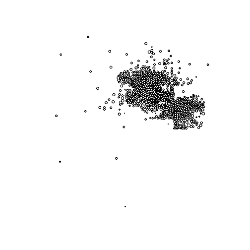
Load spatial Data
github.url <- "https://raw.githubusercontent.com/DS4PS/cpp-529-master/master/data/phx_dorling.geojson"
phx <- geojson_read(x = github.url, what = "sp")
plot(phx)
Create sub-set data frame to merge census and spatial data
# create small dataframe for the merge
df <- data.frame(tractid = d5$tractid, mhmval.00, mhmval.10, mhmval.change, pct.mhmval)


# create GEOID that matches GIS format

# create a geoID for merging by tract
df$GEOID <- substr(df$tractid, 6, 18)  # extract codes
df$GEOID <- gsub("-", "", df$GEOID)  # remove hyphens
class(df$GEOID)
[1] "character"
head(df$GEOID)
[1] "01001020100" "01001020200" "01001020300" "01001020400" "01001020500"
[6] "01001020600"
head(phx@data) # sp class from GIS file, so data frame is located @data
      GEOID2       GEOID STATEFP COUNTYFP TRACTCE             AFFGEOID   NAME
1 4013010101 04013010101      04      013  010101 1400000US04013010101 101.01
  LSAD    ALAND AWATER  POP  MHHI  ID  pop.w pnhwht12 pnhblk12 phisp12 pntv12
1   CT 54284173  27466 4915 87167 437 0.4915    95.17        0    3.64      0
  pfb12 polang12 phs12 pcol12 punemp12 pflabf12 pprof12 pmanuf12 pvet12 psemp12
1  8.22     6.68 19.82  51.53     7.56    39.43   48.52     7.44  14.89   22.66
    hinc12  incpc12 ppov12 pown12 pvac12 pmulti12  mrent12 mhmval12 p30old12
1 39.28424 23.73314   7.37  92.19   32.5     0.81 55.12244 48.42995    13.37
  p10yrs12 p18und12 p60up12 p75up12 pmar12 pwds12 pfhh12
1    74.75    14.18   41.41   17.43  82.28  10.39   0.26
 [ reached 'max' / getOption("max.print") -- omitted 5 rows ]
# merge census data with dorling map

nrow(phx)  # check dimensions
[1] 913
phx <- merge(phx, df, by.x = "GEOID", by.y = "GEOID")

# make sure they have not changed or you are missing rows in your data frame or
# merging with the wrong ID
nrow(phx)
[1] 913
Dorling Cartograms
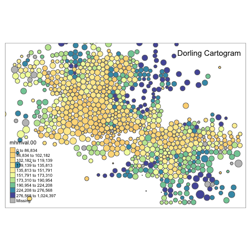
According to this Dorling Cartogram Map, high value tracts are located on the central, northeastern, and southern sides of Phoenix, Arizona.
phx <- spTransform(phx, CRS("+init=epsg:3395"))

bb <- st_bbox(c(xmin = -12519146, xmax = -12421368, ymax = 3965924, ymin = 3899074),
    crs = st_crs("+init=epsg:3395"))

tm_shape(phx, bbox = bb) + tm_polygons(col = "mhmval.00", n = 10, style = "quantile",
    palette = "Spectral") + tm_layout("Dorling Cartogram", title.position = c("right",
    "top"))
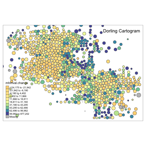
Acccording to this Dorling Cartogram Map, the largest gain from 2000-2010 occurred in the tracts that were below average in 2000.
tm_shape(phx, bbox = bb) + tm_polygons(col = "mhmval.change", n = 10, style = "quantile",
    palette = "Spectral", midpoint = NA) + tm_layout("Dorling Cartogram", title.position = c("right",
    "top"))
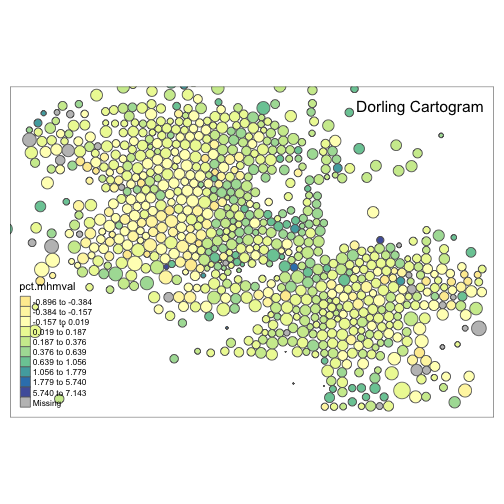
This Dorling Cartogram Map shows the percentage change in median Home values from 2000 to 2010 for Phoenix, AZ Metro Area.
tm_shape(phx, bbox = bb) + tm_polygons(col = "pct.mhmval", n = 10, style = "jenks",
    palette = "Spectral", midpoint = 0, showNA = TRUE) + tm_layout("Dorling Cartogram",
    title.position = c("right", "top"))
References
- Baum-Snow, N., & Hartley, D. (2016). Accounting for central neighborhood change, 1980-2010. Retrieved April 29, 2020, from https://github.com/DS4PS/cpp-528-spr-2020/raw/master/articles/home-value-change/economic-model-central-city-neighborhoods-white-flight-white-return.pdf