Predicting Median Home Value Change
Neighborhood change is based on many variables which measures the health of the neighborhood. Home value is considered as main variable to capture neighborhood changes because the prices of houses factor in various factors which cannot be priced directly but affect the neighborhood. This paper creates a baseline model for neighborhood analysis from 2000 -2010 using census LTDB data.
Set-Up
Library
# load Library

library(dplyr)
library(knitr)
library(pander)
library(stargazer)
library(scales)
library(here)
library(tidyr)

# set stargazer type to text for previewing in RMD docs but convert to type HTML
# when knitting (next code chunk)

s.type <- "html"
Data
# Load data

d.2000 <- readRDS(here("data/processed/LTDB-2000.rds"))
d.2010 <- readRDS(here("data/processed/LTDB-2010.rds"))
md.00.10 <- readRDS(here("data/processed/LTDB-META-DATA.rds"))

d.2000 <- select(d.2000, -year)
d.2010 <- select(d.2010, -year)

d.full <- merge(d.2000, d.2010, by = "tractid")
d.full <- merge(d.full, md.00.10, by = "tractid")
Functions
# Load helper functions

source(here("analysis/utilities/function_sg.R"))
Data Wrangling
For the purpose of the predicting Median Home Value changes from 2000 to 2010 only urban tracts are considered. House Value less than $10000 in 2000 and growth of over 200% are dropped. This is done to draw more meaningful comparison. Usually a property which is valued at less than $10,000 is vacant and growth of over 200% is marked by new developement. Including these outlier will skew the data.
Keep only urban data
# filter rural districts
table(d.full$urban.x)
rural urban
12971 59722
d.full <- filter(d.full, urban.x == "urban")
Keep a copy of data for future use
d.store <- d.full
Store original in case you need to reset anything
d.full <- d.store
Create variables to measure growth in MHV from 2000-2010.
Variables used in measuring Neigborhood Health metrics are used here.
d.full <- select(d.full, tractid, mhmval00, mhmval12, hinc00, hinc12, col00, col12,
    prof00, prof12, incpc00, incpc12, hs00, hs12, unemp00, unemp12, wds00, wds12,
    clf00, ag25up00, empclf00, empclf12, ag25up12, clf12, ag15up12, ag15up00, hu00,
    vac00, own00, rent00, h30old00, empclf00, dpov00, npov00, pop00.x, nhwht00, nhblk00,
    hisp00, asian00, cbsa.x, cbsaname.x) %>% filter(incpc00 != 0, ag25up00 != 0,
    ag25up12 != 0, empclf00 != 0, empclf12 != 0, clf00 != 0, clf12 != 0, ag15up00 !=
        0, ag15up12 != 0, prof00 != 0, col00 != 0, hs00 != 0, unemp00 != 0, wds00 !=
        0) %>% na.omit()
# !is.na()


d.full <- d.full %>% mutate(p.white = 100 * nhwht00/pop00.x, p.black = 100 * nhblk00/pop00.x,
    p.hisp = 100 * hisp00/pop00.x, p.asian = 100 * asian00/pop00.x, p.hs = 100 *
        (hs00 + col00)/ag25up00, p.hs.10 = 100 * (hs12 + col12)/ag25up12, p.col = 100 *
        col00/ag25up00, p.col.10 = 100 * col12/ag25up12, p.prof = 100 * prof00/empclf00,
    p.prof.10 = 100 * prof12/empclf12, p.unemp = 100 * unemp00/clf00, p.unemp.10 = 100 *
        unemp12/clf12, p.vacant = 100 * vac00/hu00, p.wds.00 = 100 * wds00/ag15up00,
    p.wds.10 = 100 * wds12/ag15up12, mhv.change.00.to.10 = mhmval12 - mhmval00, p.mhv.change = 100 *
        (mhmval12 - mhmval00)/mhmval00, pov.rate = 100 * npov00/dpov00) %>% filter(p.white !=
    0, p.black != 0, p.hisp != 0, p.asian != 0, p.hs != 0, p.hs.10 != 0, p.col !=
    0, p.col.10 != 0, p.prof != 0, p.prof.10 != 0, p.unemp != 0, p.unemp.10 != 0,
    p.vacant != 0, p.wds.00 != 0, p.wds.10 != 0, pov.rate != 0) %>% na.omit()

# adjust 2000 home values for inflation
mhv.00 <- d.full$mhmval00 * 1.28855
mhv.10 <- d.full$mhmval12

# change in MHV in dollars
mhv.change <- mhv.10 - mhv.00

# drop low 2000 median home values to avoid unrealistic growth rates.  tracts
# with homes that cost less than $10,000 are outliers

mhv.00[mhv.00 < 10000] <- NA

# change in MHV in percent
mhv.growth <- 100 * (mhv.change/mhv.00)

# eliminate the tracts with MHV growth of more than 200%
mhv.00[mhv.growth > 200] <- NA

d.full$mhv.00 <- mhv.00
d.full$mhv.10 <- mhv.10
d.full$mhv.change <- mhv.change
d.full$mhv.growth <- mhv.growth
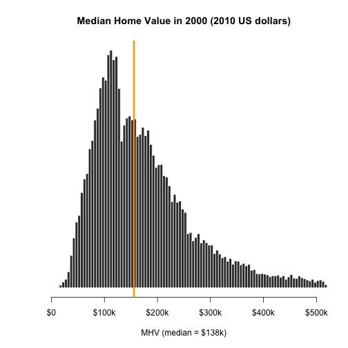
Median home value in 2000
hist(mhv.00, breaks = 200, xlim = c(0, 5e+05), col = "gray20", border = "white",
    axes = F, xlab = "MHV (median = $138k)", ylab = "", main = "Median Home Value in 2000 (2010 US dollars)")

axis(side = 1, at = seq(0, 5e+05, 1e+05), labels = c("$0", "$100k", "$200k", "$300k",
    "$400k", "$500k"))

abline(v = median(mhv.00, na.rm = T), col = "orange", lwd = 3)
Descriptive analysis of MHV in 2000 and 2010
df <- data.frame(MedianHomeValue2000 = mhv.00, MedianHomeValue2010 = mhv.10, MHV.Change.00.to.10 = mhv.change,
    MHV.Growth.00.to.10 = mhv.growth)

stargazer(df, type = s.type, digits = 0, summary.stat = c("min", "p25", "median",
    "mean", "p75", "max"))
| Statistic | Min | Pctl(25) | Median | Mean | Pctl(75) | Max |
| MedianHomeValue2000 | 12,884 | 106,692 | 155,528 | 188,060 | 225,337 | 1,288,551 |
| MedianHomeValue2010 | 9,999 | 123,100 | 191,700 | 247,026 | 314,300 | 1,000,001 |
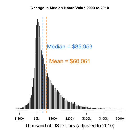
| MHV.Change.00.to.10 | -1,063,342 | 7,200 | 35,953 | 60,061 | 94,452 | 1,000,001 |
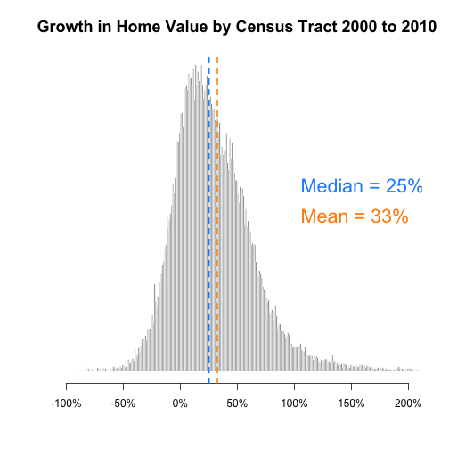
| MHV.Growth.00.to.10 | -97 | 6 | 25 | 33 | 49 | 6,059 |
Absolute changes in MHV from 2000-2010
hist(mhv.change/1000, breaks = 500, xlim = c(-100, 500), yaxt = "n", xaxt = "n",
    xlab = "Thousand of US Dollars (adjusted to 2010)", cex.lab = 1.5, ylab = "",
    main = "Change in Median Home Value 2000 to 2010", col = "gray20", border = "white")

axis(side = 1, at = seq(from = -100, to = 500, by = 100), labels = paste0("$", seq(from = -100,
    to = 500, by = 100), "k"))

mean.x <- mean(mhv.change/1000, na.rm = T)
abline(v = mean.x, col = "darkorange", lwd = 2, lty = 2)
text(x = 200, y = 1500, labels = paste0("Mean = ", dollar(round(1000 * mean.x, 0))),
    col = "darkorange", cex = 1.8, pos = 3)

median.x <- median(mhv.change/1000, na.rm = T)
abline(v = median.x, col = "dodgerblue", lwd = 2, lty = 2)
text(x = 200, y = 2000, labels = paste0("Median = ", dollar(round(1000 * median.x,
    0))), col = "dodgerblue", cex = 1.8, pos = 3)
Percent change in MHV from 2000- 2010
hg <- hist(mhv.growth, breaks = 5000, xlim = c(-100, 200), yaxt = "n", xaxt = "n",
    xlab = "", cex.main = 1.5, ylab = "", main = "Growth in Home Value by Census Tract 2000 to 2010",
    col = "gray40", border = "white")

axis(side = 1, at = seq(from = -100, to = 200, by = 50), labels = paste0(seq(from = -100,
    to = 200, by = 50), "%"))

ymax <- max(hg$count)

mean.x <- mean(mhv.growth, na.rm = T)
abline(v = mean.x, col = "darkorange", lwd = 2, lty = 2)
text(x = 100, y = (0.5 * ymax), labels = paste0("Mean = ", round(mean.x, 0), "%"),
    col = "darkorange", cex = 1.8, pos = 4)

median.x <- median(mhv.growth, na.rm = T)
abline(v = median.x, col = "dodgerblue", lwd = 2, lty = 2)
text(x = 100, y = (0.6 * ymax), labels = paste0("Median = ", round(median.x, 0),
    "%"), col = "dodgerblue", cex = 1.8, pos = 4)
Community Health
The variables used to calculate the instruments for nieghborhood changes are selected for the years 2000 and 2010. First absolute change is calculated by substracting the value of the variables in 2010 from the values in 2000. A percent change is calculated and converetd in log values to remove the skews.
# median home value in 2000, 2010, change and percentage change 2000 values
# adjusted for inflation
d.full$mhv.00 <- mhv.00
d.full$mhv.10 <- mhv.10
d.full$mhv.change <- mhv.change
d.full$mhv.growth <- mhv.growth

# Percapita income in 2000, 2010, change and percentage chnage 2000 values
# adjusted for inflation
incp.00 <- (d.full$incpc00 * 1.28855)
incpc.10 <- d.full$incpc12
incpc.change <- incpc.10 - incp.00
pct.incpc.change <- incpc.change/incp.00
pct.incpc.change <- log10(pct.incpc.change + 1)

d.full$incpc00 <- incp.00
d.full$incpc12 <- incpc.10
d.full$incpc.change <- incpc.change
d.full$pincpc.growth <- pct.incpc.change

# Median House Hold income income in 2000, 2010, change and percentage chnage
# 2000 values adjusted for inflation
hinc.00 <- d.full$hinc00 * 1.28855
hinc.10 <- d.full$hinc12
hinc.change <- hinc.10 - hinc.00
pct.hinc.change <- (hinc.change/hinc.00)
pct.hinc.change <- log10(pct.hinc.change + 1)

d.full$hinc00 <- hinc.00
d.full$hinc12 <- hinc.10
d.full$hinc.change <- hinc.change
d.full$phinc.growth <- pct.hinc.change


# % of professional employees in 2000, 2010, change and percentage chnage
pprof.00 <- d.full$p.prof
pprof.10 <- d.full$p.prof.10
pprof.change <- pprof.10 - pprof.00
pct.pprof.change <- (pprof.change/pprof.00)
pct.pprof.change <- log10(pct.pprof.change + 1)

d.full$pprof.change <- pprof.change
d.full$pprof.growth <- pct.pprof.change


# % of popualtion with High school degree or less in 2000, 2010, change and
# percentage chnage
phs.00 <- d.full$p.hs
phs.10 <- d.full$p.hs.10
phs.change <- phs.10 - phs.00
pct.phs.change <- phs.change/phs.00
pct.phs.change <- log10(pct.phs.change + 1)


d.full$phs.change <- phs.change
d.full$phs.growth <- pct.phs.change


# % of population with four years of college or more in 2000, 2010, change and
# percentage chnage
pcol.00 <- d.full$p.col
pcol.10 <- d.full$p.col.10
pcol.change <- pcol.10 - pcol.00
pct.pcol.change <- pcol.change/pcol.00
pct.pcol.change <- log10(pct.pcol.change + 1)


d.full$pcol.change <- pcol.change
d.full$pcol.growth <- pct.pcol.change

# % of unemployed population in 2000, 2010, change and percentage chnage
punemp.00 <- d.full$p.unemp
punemp.10 <- d.full$p.unemp.10
punemp.change <- punemp.10 - punemp.00
pct.punemp.change <- punemp.change/punemp.00
pct.punemp.change <- log10(pct.punemp.change + 1)

d.full$punemp.change <- punemp.change
d.full$punemp.growth <- pct.punemp.change

# % of widowed, divorced and single population in 2000, 2010, change and
# percentage chnage
pwds.00 <- d.full$p.wds.00
pwds.10 <- d.full$p.wds.10
pwds.change <- pwds.10 - pwds.00
pct.pwds.change <- pwds.change/pwds.00
pct.pwds.change <- log10(pct.pwds.change + 1)

d.full$pwds.change <- pwds.change
d.full$pwds.growth <- pct.pwds.change
Measures
Instrument 1
Measures Economic wealth of the community. The variables included in the instruments are:
- Median home value mhmval and mhmval12
- Percent professional employees
- Median HH Income, total
Instrument 2
Measure Human Capital of the neighborhood. The variables included in the instruments are:
- Median home value
- % with 4 years college degree or more
- per capita income
Instrument 3
Measures the Hardship faced by the neighborhood. The variables included in the instruments are:
- Median home value
- % high school degree or less
- Median HH income
Instrument 4
Measures the distress in a neighborhood. The variable included in the instrument are:
- Median home value
- Median HH Income, total
- Percent unemployed
- Percent widowed, divorced and seperated
# Instrument 1 Economic wealth Median home value mhmval and mhmval12.  percent
# professional employees Median HH Income, total

df.instrument1 <- select(d.full, PercentGrowthMedianHomeValue.00.to.10 = mhv.growth,
    PercentProfessionalChange.00to.10 = pprof.growth, PercentHouseHoldIncome = phinc.growth) %>%
    na.omit()


# Instrument 2 Human Capital Median home value % with 4 years college degree or
# more per capita income

df.instrument2 <- select(d.full, PercentGrowthMedianHomeValue.00.to.10 = mhv.growth,
    PercentWithFourYearCollegeDegreeOrMoreChange00.to.10 = pcol.growth, PercaptiaIncomeChange.00.to.10 = pincpc.growth) %>%
    na.omit()


# Instrument 3 Hardship index Median home value % high school degree or less
# median HH income

df.instrument3 <- select(d.full, PercentGrowthMedianHomeValue.00.to.10 = mhv.growth,
    PercentWithHighSchoolDegreeOrLessChange.00.to.10 = phs.growth, HouseHoldIncomeChange.00.to.10 = phinc.growth) %>%
    na.omit()

## Instrument 4 ditressed neighborhood Median home value Median HH Income, total
## percent unemployed percent widowed, divorced and seperated

df.instrument4 <- select(d.full, PercentGrowthMedianHomeValue.00.to.10 = mhv.growth,
    Percentunemployed.00.to.10 = punemp.growth, HouseHoldIncomeChange.00.to.10 = phinc.growth,
    PercentWidowedDivorcedChange.00.to.10 = pwds.growth) %>% na.omit()
Bivariate Correlation
Bivariate correlation shows the relationship between individual variables in an instrument. This is a great way to assess relationships visually.
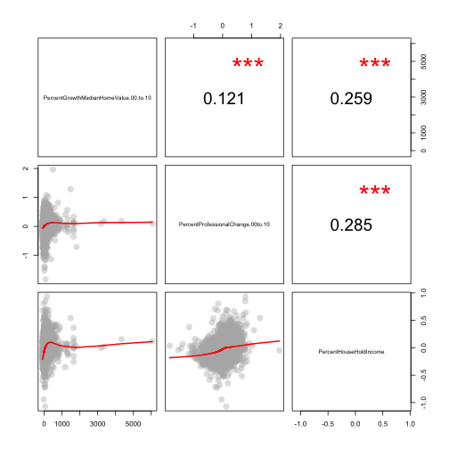
Instrument 1 - Economic wealth - Bivariate Correlation
This instrument measures economic wealth by measuring the changes in professional population and household income against the changes in Home values in the neighborhood.
set.seed(1234)
pairs(df.instrument1, lower.panel = panel.smooth, upper.panel = panel.cor)
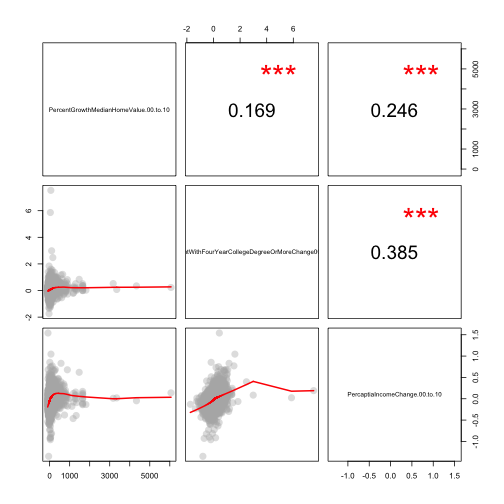
Instrument 2 - Human Capital - Bivariate Correlation
This instrument measures Human Capital by measuring the changes in per capita income and college-educated population against the changes in Home values in the neighborhood.
pairs(df.instrument2, lower.panel = panel.smooth, upper.panel = panel.cor)
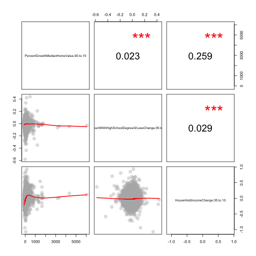
Instrument 3 - Hardship Index - Bivariate Correlation
This instrument measures Hardship Index by measuring the changes in population with less than High School education and Household Income against the changes in Home values in the neighborhood.
pairs(df.instrument3, lower.panel = panel.smooth, upper.panel = panel.cor)
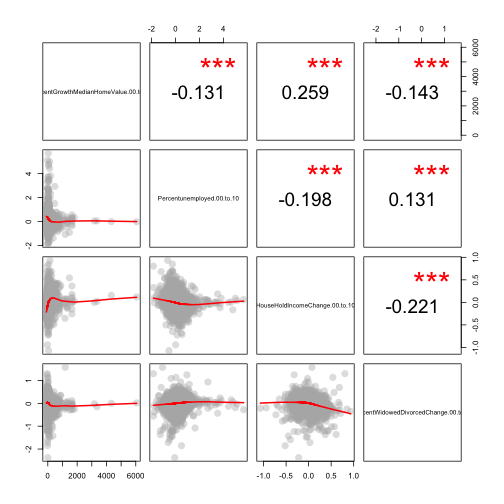
Instrument 4 - Distress Index - Bivariate Correlation
This instrument measures neighborhood distress by measuring the changes in unemployed Population, Household Income and divorced, wodowed population against the changes in Home values in the neighborhood.
pairs(df.instrument4, lower.panel = panel.smooth, upper.panel = panel.cor)
Regression Analysis
A regression analysis with all four metrices of community health is shown below. All the models have a P value of low value of less than .00001 making them significant. A closer look reveals that model 1 which also measures Economic Wealth of the community is describes the neighborhood health best because of low standard errors of the varibales. Including percentage of unemployed population in my opinion is can improve the model further. This confirms my intial obeservation as the Economic Wealth Index has the highest Cornbach Alpha score amongst all four.
reg.ch1 <- lm(mhv.growth ~ pprof.growth + phinc.growth, data = d.full)

reg.ch2 <- lm(mhv.growth ~ pcol.growth + pincpc.growth, data = d.full)

reg.ch3 <- lm(mhv.growth ~ phinc.growth + phs.growth, data = d.full)

reg.ch4 <- lm(mhv.growth ~ phinc.growth + punemp.growth + pwds.growth, data = d.full)

stargazer(reg.ch1, reg.ch2, reg.ch3, reg.ch4, type = s.type, dep.var.labels = ("Median Home Value change 2000-2010"),
    column.labels = c("Economic Wealth", "Human Capital", "Hardship Index", "Distress Index"),
    digits = 2)
| Dependent variable: | ||||
| Median Home Value change 2000-2010 | ||||
| Economic Wealth | Human Capital | Hardship Index | Distress Index | |
| (1) | (2) | (3) | (4) | |
| pprof.growth | 26.27*** | |||
| (2.15) | ||||
| phinc.growth | 176.01*** | 186.16*** | 162.44*** | |
| (3.01) | (2.89) | (2.98) | ||
| pcol.growth | 35.21*** | |||
| (1.76) | ||||
| pincpc.growth | 156.92*** | |||
| (3.20) | ||||
| phs.growth | 26.04*** | |||
| (6.88) | ||||
| punemp.growth | -16.48*** | |||
| (0.89) | ||||
| pwds.growth | -42.79*** | |||
| (2.10) | ||||
| Constant | 35.90*** | 31.32*** | 36.78*** | 40.68*** |
| (0.27) | (0.29) | (0.27) | (0.34) | |
| Observations | 58,202 | 58,202 | 58,202 | 58,202 |
| R2 | 0.07 | 0.07 | 0.07 | 0.08 |
| Adjusted R2 | 0.07 | 0.07 | 0.07 | 0.08 |
| Residual Std. Error | 62.28 (df = 58199) | 62.35 (df = 58199) | 62.35 (df = 58199) | 61.91 (df = 58198) |
| F Statistic | 2,166.78*** (df = 2; 58199) | 2,092.02*** (df = 2; 58199) | 2,094.51*** (df = 2; 58199) | 1,689.97*** (df = 3; 58198) |
| Note: | *p<0.1; **p<0.05; ***p<0.01 | |||
Predict MHV Change
Each city is unique in terms of its history, culture, people, vibe, political stability, economies, geography and climate. These factors cannot be ignored while measuring or predicting changes in Home values. Census data cannot track all these different attributes. However, the data can be brought to reflects metro based attributes by metro-level fixed effect to the model. Introducing average median home value growth of the metro area as a control variable will take care of the issue. This helps in anchoring dependent variable which is home value in this case.
In this case Fixed effect model is a good fit because it has higher adjusted R2. Home values responds differently to changes in household income, Professional population and unemployed population.For eg; for each percentage change in unemployed population home value changes decrease by 6.98 % in fixed effect model whereas the home value decreases by 9.50 % when we don't account for metro effect.
# Three variables phinc.growth, pprof.growth, punemp.growth


df.ch.mhv <- d.full %>%
  group_by( cbsaname.x ) %>%
  mutate( metro.mhv.growth = 100 * median( mhv.growth,na.rm = T ) ) %>%
  ungroup() %>%
  na.omit()


 reg.ch.mhv.fe <- lm (mhv.growth ~ phinc.growth + pprof.growth + punemp.growth + metro.mhv.growth + cbsa.x, data = df.ch.mhv )

 reg.ch.mhv <- lm (mhv.growth ~ phinc.growth + pprof.growth + punemp.growth , data = df.ch.mhv )

 stargazer( reg.ch.mhv, reg.ch.mhv.fe,
           type=s.type, digits=2,
           dep.var.labels = ("Median Home Value change 2000-2010"),
           column.labels = c( "No Fixed Effect", "Metro Fixed Effect Model"),
           #omit.stat = c("rsq","f"),
           omit="cbsa.x",
          add.lines = list(c("Metro Fixed Effects:", "NO","YES"))
 )
| Dependent variable: | ||
| Median Home Value change 2000-2010 | ||
| No Fixed Effect | Metro Fixed Effect Model | |
| (1) | (2) | |
| phinc.growth | 145.02*** | 77.95*** |
| (1.58) | (1.33) | |
| pprof.growth | 16.55*** | 28.45*** |
| (1.11) | (0.89) | |
| punemp.growth | -11.97*** | -7.16*** |
| (0.45) | (0.38) | |
| metro.mhv.growth | 0.02*** | |
| (0.004) | ||
| Constant | 35.51*** | -10.02 |
| (0.18) | (10.53) | |
| Metro Fixed Effects: | NO | YES |
| Observations | 57,748 | 57,748 |
| R2 | 0.18 | 0.49 |
| Adjusted R2 | 0.18 | 0.49 |
| Residual Std. Error | 31.59 (df = 57744) | 24.92 (df = 57366) |
| F Statistic | 4,110.95*** (df = 3; 57744) | 145.13*** (df = 381; 57366) |
| Note: | *p<0.1; **p<0.05; ***p<0.01 | |