Evaluating Federal Programs

CPP 528 Final Project Spring 2020

Federal Program Data

Evaluation of Tax Credit Programs

Throughout this report we have explored various measures of gentrification in the United States and identified ways to predict which communities are at risk. However, once we have discovered vulnerable areas, how can we effect change through policymaking?

Over the last several decades, the federal government has devised two primary strategies to strengthen communities and reduce the effects of gentrification: Supply-Side Mechanisms and Demand-Side Mechanisms (Lecy, 2020). Both mechanisms aim to improve communities by incentivizing investors to develop low-income and high-risk areas and subsequently have resulted in two different tax credit programs: The Low-Income Housing Tax Credit for the Supply-Side Mechanism and the New Market Tax Credit for the Demand-Side Mechanism.

What is the Low-Income Housing Tax Credit (LIHTC) Program?

The LIHTC program was created by the Tax Reform Act of 1986 and operates on an annual budget of nearly $8 billion dollars (HUD, 2019; Lecy, 2020). The primary goal of the LIHTC is to motivate investors to acquire, rehabilitate, and construct rental housing for low and moderate income tenants in areas that have high costs (HUD, 2019; Tax Policy Center, n.d.a). Tax credits are issued to state and territorial governments that then utilize a competitive application process to award the credits to developers (Tax Policy Center, n.d.a). Afterwards, these developers often sell the credits to private investors who then claim the credits in their taxes once their housing development becomes available to house tenants (Tax Policy Center, n.d.a).

What is the New Market Tax Credit (NMTC) Program?

The NMTC program was created by the Community Renewal Tax Relief Act of 2000 (Lecy, 2020). Although its operating costs fluctuate, they average at around $1.3 billion dollars anually (Tax Policy Center, n.d.b). The primary goal of the NMTC is to encourage developers and investors to bring businesses in the manufacturing, food, retail, housing, health, technology, energy, education, and childcare sectors to economically distressed communities (CDFI Fund, 2018). The federal Community Development Financial Institutions Fund (CDFI) uses a competitive application process to distribute tax credits to Community Development Entities (CDEs) who then offer the credits to investors in exchange for equity (CDFI Fund, 2018).

Which areas are eligible for the LIHTC vs NMTC?

The federal government established both tax credit programs with the common goal of improving disadvantaged communities. However, the eligibility guidelines for the programs differ.

The LIHTC program does not have specific guidelines for what constitutes as a property for lower-income and disadvantaged populations. However, there are requirements that rent can only cost 30% of the average income of the area (PD&R Edge, 2017). According to Novogradac (2016), "[t]ax credit housing is generally located where the land costs are lower and the tax credit allowable rents are sufficient to allow for market-rate rents".

In contrast, the NMTC program defines disadvantaged communities as "census tracts with a poverty rate of 20 percent or greater, or a median family income at or below 80 percent of the applicable area median family income" or investments that meet "statutory provisions designed to target certain areas or populations, including provisions for Rural Counties, and Low-Income Targeted Populations" (CDFI Fund, 2019). The Tax Policy Center (n.d.b) reports that "all applicants have pledged to place at least 75 percent of their NMTC projects in “severely distressed” census tracts".

Data Analytics

Through the following statistical tools and data analytics, we attempt to explore the impact of these programs on areas vulnerable for gentrification and determine which of these approaches result in neighborhood growth.

Set-Up

Library

library(knitr)
library(pander)
library(stargazer)
library(scales)
library(ggplot2)
library(gridExtra)
library(here)
library(tidyverse)

set.seed(1234)

# set stargazer type to text for previewing in RMD docs but convert to type HTML
# when knitting (next code chunk)

s.type <- "html"

Data

# Load Rodeo Data with merged Low Income Housing Tax Credit, New Market Tax
# Credit, and Census Data

d <- readRDS(here("/data/rodeo/merged-lihtc-nmtc-census-data.rds"))

Census Data Descriptives

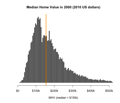
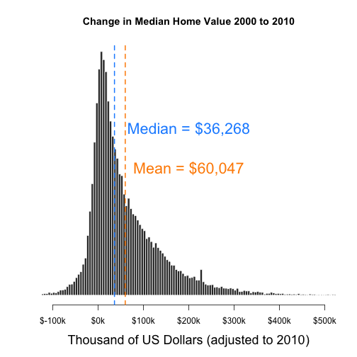
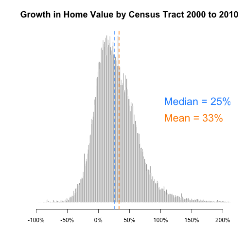
The following images and table display summary statistics of changes and growth in median home value from 2000 to 2010.

Median Home Value: Histogram

us.median <- paste0("$", round(median(d$mhv.00/1000, na.rm = T), 0), "k")

hist(d$mhv.00, breaks = 200, xlim = c(0, 5e+05), col = "gray20", border = "white",
    axes = F, xlab = paste0("MHV (median = ", us.median, ")"), ylab = "", main = "Median Home Value in 2000 (2010 US dollars)")

axis(side = 1, at = seq(0, 5e+05, 1e+05), labels = c("$0", "$100k", "$200k", "$300k",
    "$400k", "$500k"))

abline(v = median(d$mhv.00, na.rm = T), col = "orange", lwd = 3)

Median Home Value: Table

df <- data.frame(MedianHomeValue2000 = d$mhv.00, MedianHomeValue2010 = d$mhv.10,
    MHV.Change.00.to.10 = d$mhv.change, MHV.Growth.00.to.12 = d$mhv.growth)

stargazer(df, type = s.type, digits = 0, summary.stat = c("min", "p25", "median",
    "mean", "p75", "max"))


Statistic	Min	Pctl(25)	Median	Mean	Pctl(75)	Max

MedianHomeValue2000	11,167	105,661	154,903	187,129	224,337	1,288,551
MedianHomeValue2010	9,999	123,200	193,200	246,570	312,000	1,000,001
MHV.Change.00.to.10	-1,228,651	7,187	36,268	60,047	94,881	1,000,001
MHV.Growth.00.to.12	-97	6	25	33	50	6,059

Change in MHV 2000-2010

hist(d$mhv.change/1000, breaks = 500, xlim = c(-100, 500), yaxt = "n", xaxt = "n",
    xlab = "Thousand of US Dollars (adjusted to 2010)", cex.lab = 1.5, ylab = "",
    main = "Change in Median Home Value 2000 to 2010", col = "gray20", border = "white")

axis(side = 1, at = seq(from = -100, to = 500, by = 100), labels = paste0("$", seq(from = -100,
    to = 500, by = 100), "k"))

mean.x <- mean(d$mhv.change/1000, na.rm = T)
abline(v = mean.x, col = "darkorange", lwd = 2, lty = 2)
text(x = 200, y = 1500, labels = paste0("Mean = ", dollar(round(1000 * mean.x, 0))),
    col = "darkorange", cex = 1.8, pos = 3)

median.x <- median(d$mhv.change/1000, na.rm = T)
abline(v = median.x, col = "dodgerblue", lwd = 2, lty = 2)
text(x = 200, y = 2000, labels = paste0("Median = ", dollar(round(1000 * median.x,
    0))), col = "dodgerblue", cex = 1.8, pos = 3)

Percent Change in MHV 2000 to 2010

hg <- hist(d$mhv.growth, breaks = 5000, xlim = c(-100, 200), yaxt = "n", xaxt = "n",
    xlab = "", cex.main = 1.5, ylab = "", main = "Growth in Home Value by Census Tract 2000 to 2010",
    col = "gray40", border = "white")

axis(side = 1, at = seq(from = -100, to = 200, by = 50), labels = paste0(seq(from = -100,
    to = 200, by = 50), "%"))

ymax <- max(hg$count)

mean.x <- mean(d$mhv.growth, na.rm = T)
abline(v = mean.x, col = "darkorange", lwd = 2, lty = 2)
text(x = 100, y = (0.5 * ymax), labels = paste0("Mean = ", round(mean.x, 0), "%"),
    col = "darkorange", cex = 1.8, pos = 4)

median.x <- median(d$mhv.growth, na.rm = T)
abline(v = median.x, col = "dodgerblue", lwd = 2, lty = 2)
text(x = 100, y = (0.6 * ymax), labels = paste0("Median = ", round(median.x, 0),
    "%"), col = "dodgerblue", cex = 1.8, pos = 4)

Program Participation Criteria

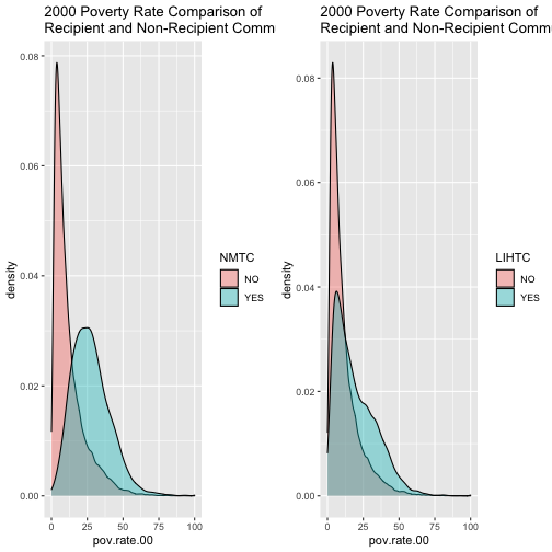
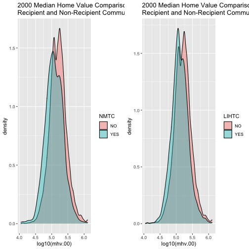
The following data examines differences in median home value for census tracts in NMTC and LIHTC eligible areas.

Create separate data sets for NMTC and LIHTC programs.

# Create a true/false code for recipient tracts
d$LIHTC <- ifelse(d$num.lihtc > 0, "YES", "NO")
d$NMTC <- ifelse(d$num.nmtc > 0, "YES", "NO")

### POVERTY RATES

plot1 <- ggplot(d, aes(x = pov.rate.00, fill = NMTC)) + geom_density(alpha = 0.4) +
    ggtitle("2000 Poverty Rate Comparison of \nRecipient and Non-Recipient Communities")

plot2 <- ggplot(d, aes(x = pov.rate.00, fill = LIHTC)) + geom_density(alpha = 0.4) +
    ggtitle("2000 Poverty Rate Comparison of \nRecipient and Non-Recipient Communities")

grid.arrange(plot1, plot2, nrow = 1)

### HOME VALUES

plot3 <- ggplot(d, aes(x = log10(mhv.00), fill = NMTC)) + geom_density(alpha = 0.4) +
    ggtitle("2000 Median Home Value Comparison of \nRecipient and Non-Recipient Communities")

plot4 <- ggplot(d, aes(x = log10(mhv.00), fill = LIHTC)) + geom_density(alpha = 0.4) +
    ggtitle("2000 Median Home Value Comparison of \nRecipient and Non-Recipient Communities")

grid.arrange(plot3, plot4, nrow = 1)

Household Income Comparison in 2000: Program Recipients vs Non-Recipient Tracts

### HOUSEHOLD INCOME COMPARISON IN 2000: PROGRAM RECIPIENTS VS NON-RECIPIENT TRACTS

# Tracts that received LIHTC
mean(d$hinc00[d$num.lihtc > 0])

[1] 47214.89

# Tracts that did not
mean(d$hinc00[d$num.lihtc == 0])

[1] 63671.74

# Tracts that received NMTC
mean(d$hinc00[d$num.nmtc > 0])

[1] 35677.12

# Tracts that did not
mean(d$hinc00[d$num.nmtc == 0])

[1] 62164.61

Home Value 2000:

### MEDIAN HOME VALUE COMPARISON IN 2000

# Tracts that received LIHTC
mean(d$mhv.00[d$num.lihtc > 0], na.rm = T)

[1] 156465.4

# Tracts that did not
mean(d$mhv.00[d$num.lihtc == 0], na.rm = T)

[1] 192012.7

# Tracts that received NMTC
mean(d$mhv.00[d$num.nmtc > 0], na.rm = T)

[1] 146649

# Tracts that did not
mean(d$mhv.00[d$num.nmtc == 0], na.rm = T)

[1] 188304.4

Poverty Rates 2000:

### POVERTY RATE COMPARISONS

# Tracts that received LIHTC
summary(d$pov.rate.00[d$num.lihtc > 0])

   Min. 1st Qu.  Median    Mean 3rd Qu.    Max.    NA's 
  0.000   7.989  15.919  19.440  28.628  88.210       6

# Tracts that did not
summary(d$pov.rate.00[d$num.lihtc == 0])

   Min. 1st Qu.  Median    Mean 3rd Qu.    Max.    NA's 
  0.000   4.145   7.785  11.293  14.768 100.000     182

# Tracts that received NMTC
summary(d$pov.rate.00[d$num.nmtc > 0])

   Min. 1st Qu.  Median    Mean 3rd Qu.    Max.    NA's 
   0.00   17.79   26.13   27.49   35.14   93.17       3

# Tracts that did not
summary(d$pov.rate.00[d$num.nmtc == 0])

   Min. 1st Qu.  Median    Mean 3rd Qu.    Max.    NA's 
  0.000   4.335   8.240  11.973  15.835 100.000     185

Plot

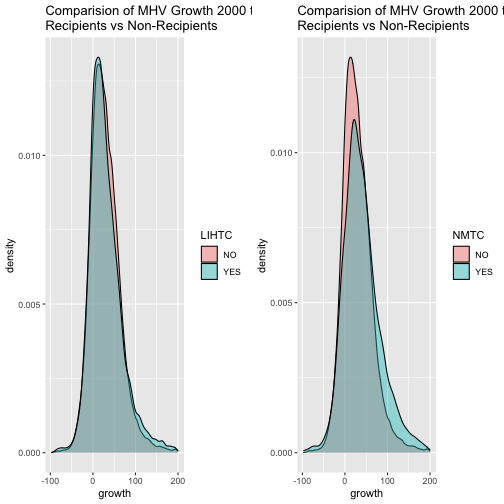
### MHV Growth Rates (DV in Model)

d$growth <- d$mhv.growth
d$growth[d$growth > 200] <- NA

p5 <- ggplot(d, aes(x = growth, fill = LIHTC)) + geom_density(alpha = 0.4) + ggtitle("Comparision of MHV Growth 2000 to 2010: \nRecipients vs Non-Recipients")

p6 <- ggplot(d, aes(x = growth, fill = NMTC)) + geom_density(alpha = 0.4) + ggtitle("Comparision of MHV Growth 2000 to 2010: \nRecipients vs Non-Recipients")

grid.arrange(p5, p6, nrow = 1)

Summary Statistics of Eligible and Ineligible Census Tracts

# Tracts that received LIHTC
summary(d$growth[d$num.lihtc > 0])

   Min. 1st Qu.  Median    Mean 3rd Qu.    Max.    NA's 
-88.967   4.233  23.027  29.885  48.869 199.739     155

# Tracts that did not
summary(d$growth[d$num.lihtc == 0])

   Min. 1st Qu.  Median    Mean 3rd Qu.    Max.    NA's 
-96.891   5.981  25.332  29.398  48.725 199.550     611

# Tracts that received NMTC
summary(d$growth[d$num.nmtc > 0])

   Min. 1st Qu.  Median    Mean 3rd Qu.    Max.    NA's 
 -94.55   10.94   33.36   39.60   62.96  199.31      82

# Tracts that did not
summary(d$growth[d$num.nmtc == 0])

   Min. 1st Qu.  Median    Mean 3rd Qu.    Max.    NA's 
-96.891   5.609  24.834  29.177  48.391 199.739     684

Evaluating Program Impact

The following regression anyalses examine differences in program impact of the NMTC and LIHTC programs.

options(scipen = 999)

y1 <- log(d$mhv.00)
y2 <- log(d$mhv.10)
treat.nmtc <- as.numeric(d$num.nmtc > 0)
treat.lihtc <- as.numeric(d$num.lihtc > 0)
socialstat <- d$metro.socstat.change
diversity <- d$metro.diversity.change
neighval <- d$metro.neighval.change

d1 <- data.frame(y = y1, treat = treat.nmtc, post = 0, socialstat, diversity, neighval)
d2 <- data.frame(y = y2, treat = treat.nmtc, post = 1, socialstat, diversity, neighval)
d3 <- rbind(d1, d2)

nmtc.reg <- lm(y ~ treat + post + treat * post, data = d3)  # NMTC Regression

e1 <- data.frame(y = y1, treat = treat.lihtc, post = 0, socialstat, diversity, neighval)
e2 <- data.frame(y = y2, treat = treat.lihtc, post = 1, socialstat, diversity, neighval)
e3 <- rbind(e1, e2)

lihtc.reg <- lm(y ~ treat + post + treat * post, data = e3)  # LIHTC Regression

Summary of NMTC regression analysis

summary(nmtc.reg)

Call:
lm(formula = y ~ treat + post + treat * post, data = d3)

Residuals:
     Min       1Q   Median       3Q      Max 
-2.98214 -0.42156 -0.00984  0.40743  2.37285 

Coefficients:
             Estimate Std. Error  t value             Pr(>|t|)    
(Intercept) 11.961097   0.002650 4514.395 < 0.0000000000000002 ***
treat       -0.264915   0.015771  -16.798 < 0.0000000000000002 ***
post         0.231278   0.003745   61.765 < 0.0000000000000002 ***
treat:post   0.102738   0.022227    4.622            0.0000038 ***
---
Signif. codes:  0 '***' 0.001 '**' 0.01 '*' 0.05 '.' 0.1 ' ' 1

Residual standard error: 0.6372 on 119220 degrees of freedom
  (220 observations deleted due to missingness)
Multiple R-squared:  0.03569,	Adjusted R-squared:  0.03567 
F-statistic:  1471 on 3 and 119220 DF,  p-value: < 0.00000000000000022

Summary of LIHTC regression analysis

summary(lihtc.reg)

Call:
lm(formula = y ~ treat + post + treat * post, data = e3)

Residuals:
     Min       1Q   Median       3Q      Max 
-3.00503 -0.41782 -0.00951  0.40339  2.29453 

Coefficients:
             Estimate Std. Error t value            Pr(>|t|)    
(Intercept) 11.982150   0.002800 4279.80 <0.0000000000000002 ***
treat       -0.207651   0.007553  -27.49 <0.0000000000000002 ***
post         0.233122   0.003957   58.92 <0.0000000000000002 ***
treat:post   0.007467   0.010672    0.70               0.484    
---
Signif. codes:  0 '***' 0.001 '**' 0.01 '*' 0.05 '.' 0.1 ' ' 1

Residual standard error: 0.6344 on 119220 degrees of freedom
  (220 observations deleted due to missingness)
Multiple R-squared:  0.04426,	Adjusted R-squared:  0.04423 
F-statistic:  1840 on 3 and 119220 DF,  p-value: < 0.00000000000000022

Output of NMTC regression analysis

# Summary of New Market Tax Credit Program (NMTC)

b0 <- nmtc.reg$coefficients[1]
b1 <- nmtc.reg$coefficients[2]
b2 <- nmtc.reg$coefficients[3]
b3 <- nmtc.reg$coefficients[4]

# C1 = B0
exp(b0)

(Intercept) 
   156544.8

# C2 = B0 + B2
exp(b0 + b2)

(Intercept) 
   197279.2

# T1 = B0 + B1
exp(b0 + b1)

(Intercept) 
   120112.3

# T2 = B0 + B1 + B2 + B3
exp(b0 + b1 + b2 + b3)

(Intercept) 
   167744.7

Output of LIHTC regression analysis

# Summary of Low-Income Housing Tax Credit (LIHTC)

b0 <- lihtc.reg$coefficients[1]
b1 <- lihtc.reg$coefficients[2]
b2 <- lihtc.reg$coefficients[3]
b3 <- lihtc.reg$coefficients[4]

# C1 = B0
exp(b0)

(Intercept) 
   159875.5

# C2 = B0 + B2
exp(b0 + b2)

(Intercept) 
   201848.3

# T1 = B0 + B1
exp(b0 + b1)

(Intercept) 
   129897.3

# T2 = B0 + B1 + B2 + B3
exp(b0 + b1 + b2 + b3)

(Intercept) 
     165229

Model Evaluation

Now, we will evaluate the effectiveness of the NMTC and LIHTC programs in producing home value growth after controlling for social status (professional employee population, homeowner population, and married population), diversity (non-Hispanic White population, population living in poverty, and population with household head living in home for less than 10 years), and neighborhood value (median home value, income per capita, and college-educated population)

nmtc.reg2 <- lm(y ~ treat + post + treat * post + socialstat + diversity + neighval,
    data = d3)
lihtc.reg2 <- lm(y ~ treat + post + treat * post + socialstat + diversity + neighval,
    data = e3)

stargazer(nmtc.reg2, lihtc.reg2, type = s.type, column.labels = c("NMTC", "LIHTC"),
    covariate.labels = c("intercept (b0)", "treat (b1)", "post (b2)", "social status",
        "diversity", "neighborhood value", "treat x post (b3)"), digits = 2, intercept.bottom = FALSE)


	Dependent variable:

	y
	NMTC	LIHTC
	(1)	(2)

intercept (b0)	11.38^***	11.40^***
	(0.01)	(0.01)

treat (b1)	-0.32^***	-0.20^***
	(0.01)	(0.01)

post (b2)	0.23^***	0.23^***
	(0.003)	(0.004)

social status	6.53^***	6.47^***
	(0.10)	(0.10)

diversity	-7.11^***	-7.02^***
	(0.11)	(0.11)

neighborhood value	2.98^***	2.97^***
	(0.02)	(0.02)

treat x post (b3)	0.10^***	0.01
	(0.02)	(0.01)


Observations	119,224	119,224
R²	0.24	0.24
Adjusted R²	0.24	0.24
Residual Std. Error (df = 119217)	0.57	0.56
F Statistic (df = 6; 119217)	6,188.74^***	6,408.17^***

Note:	^p<0.1; ^p<0.05; ^**p<0.01

Are the programs effective at catalyzing neighborhood improvement?

According to this regression model, the New Market Tax Credit Program is effective at increasing growth as indicated by `b3`. This variable finds that neighborhood values increase by 10% under this program. In contrast, the LIHTC program does not display statistical significance in growth when changes in social status, diversity, and neighborhood value indexes are controlled for. Therefore, for our purposes, we find that the NMTC program is most effective.

However, it is important to also consider that census tracts in the LIHTC program may not be in need of as much growth since the goal of the program is primarily to provide lower-income residents with affordable housing in areas where they may have been displaced due to gentrification rather than to improve the surrounding neighborhood in the way that the NMTC program is designed to do. Both programs may be effective when examined through a lens other than home value growth.

References

CDFI Fund. (2018, January). NMTC program fact sheet. Retrieved April 30, 2020, from https://www.cdfifund.gov/Documents/NMTC%20Fact%20Sheet_Jan2018.pdf
CDFI Fund. (2019, November 25). CDFI Fund releases summary report and public data for NMTC program for fys 2003-2017. Retrieved April 30, 2020, from https://www.cdfifund.gov/news-events/news/Pages/news-detail.aspx?NewsID=364&Category=Press%20Releases
HUD. (2019, May 24). Low-income housing tax credits: HUD user. Retrieved April 30, 2020, from https://www.huduser.gov/portal/datasets/lihtc.html
Lecy, J. (2020). Economic development through tax credits: The NMTC and LIHTC programs. Retrieved April 30, 2020, from https://ds4ps.org/cpp-528-spr-2020/lectures/NMTC-and-LIHTC-overview.pdf
Novogradac. (2016, March 11). About the LIHTC. Retrieved April 30, 2020, from https://www.novoco.com/resource-centers/affordable-housing-tax-credits/lihtc-basics/about-lihtc
PD&R Edge. (2017, August 14). Defining housing affordability: HUD USER. Retrieved April 30, 2020, from https://www.huduser.gov/portal/pdredge/pdr-edge-featd-article-081417.html
Tax Policy Center. (n.d.). What is the low-income housing tax credit and how does it work? Retrieved April 30, 2020, from https://www.taxpolicycenter.org/sites/default/files/briefing-book/what_is_the_low-income_housing_credit_and_how_does_it_work.pdf
Tax Policy Center. (n.d.). What is the new markets tax credit, and how does it work? Retrieved April 30, 2020, from https://www.taxpolicycenter.org/sites/default/files/briefing-book/what_is_the_new_markets_tax_credit_and_how_does_it_work.pdf